Our project is a bipedal humanoid robot. Bipedal humanoid robots are robots that mimic human walking gait. The purpose for mimicking human gait is to create humanoid robots that can help humans in different jobs and tasks such as senior care in nursing homes, constructions, hazardous jobs that need humans and in general for a better human robot interaction. This bipedal humanoid robotics is a research topic that has been very popular and we can see so many different examples some of them being ASIMO, HRP and ATLAS.
Meet Our Team
HUSEYIN CEM YUMUK
ULAS BERK KARLI
YAHYA MUHAMMED KANCAL
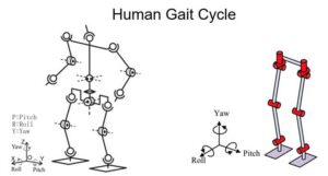
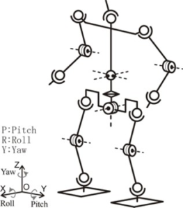
Human walking gait is a cycle and the concept of DOF (Degrees Of Freedom) is a very important concept in understanding of the human walking gait. Degrees of freedom can be stated as the number of parameters that are needed for defining the position of a particle or a rigid body. An example would be a slider on a bar, this system has only one degree of freedom because its position can be defined using only one parameter. Humans and humanoid robots in general consist of 12 degrees of freedom at total.
This creates some computational and control problems. This is because of the gait cycles landing phase. When the leg that has been raised is started being lowered until it touches the ground there must be calculations, corrections and control of the ankle so that when the foot contacts with the ground toe or heel landing of the leg is avoided. A toe or heel landing would cause a instability of the gait and humanoid robot would fall. To avoid this problem and the simplify the control of the humanoid robot we eliminated 1 degree of freedom from each leg leaving the entire humanoid robot with 10 degrees of freedom.

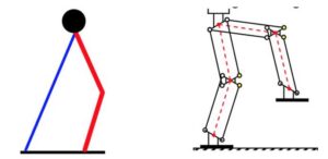
Also a system is need to be used for the movement with 10 degrees of freedom. For this system Parallel Double Crank Mechanism, which is a specialized version of the four bar mechanism.
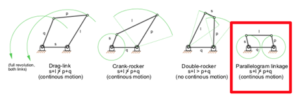
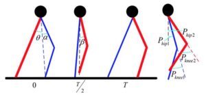
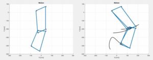
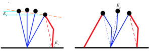
The speciality of the parallel double crank mechanism is that the two opposite links are parallel at all times thus creating two circular trajectories that can be specified as cranks.
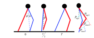
For the creation of a stable gait cycle the commonly known technique is the passive dynamic walking. We used another technique known as virtual slope walking. The Passive Dynamic Walking is a concept of using lowest possible energy from outsource. Our technique is inspired by this passive dynamic walking. There is another technique called ZMP (Zero Moment Point) which utilizes the exact time the foot hits the ground and assumes that the surface is perfectly flat and has very high friction. Compared to this our technique has far less artificial constraints and much more efficient in real-time applications.
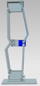
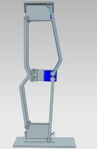
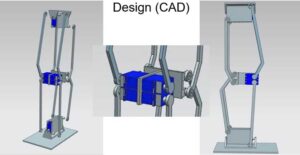
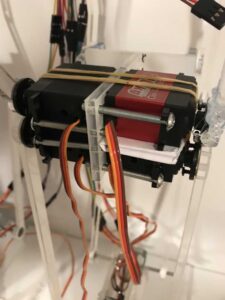
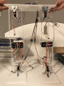
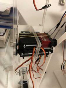
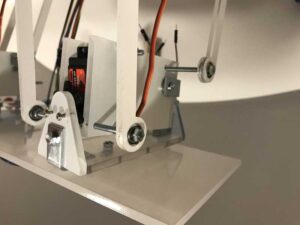
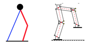
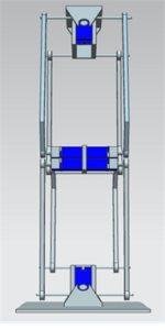
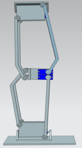
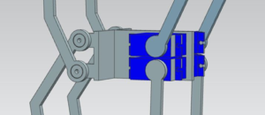
After deciding that the most appropriate mechanism to mimic a real human leg is through making use of parallel double crank mechanism, we made some research to find out how we can implement such a system to a leg. We have observed that thigh and shank portions of a human leg are almost equal to each other. That is why in our design process, we have taken this information into account. During design process we have also decided which servo motors to use on the humanoid robot. When we decide which servo motors to use, we considered their weight and maximum torque that they can produce. After deciding which servo motor to use, we have looked at their data sheets to get their dimensions. According to their dimensions, we have designed the components of humanoid robot which are responsible of holding the servo motors. We could predict that when we connect servo motor holders to the links that connects other servo motor holders to each other there might occur friction on the connection surfaces. Because of this reason, we decided to use regular ball bearings to reduce friction between surfaces. Finally, to balance the humanoid leg, we needed to make the surface of the feet large and we designed the feet accordingly.
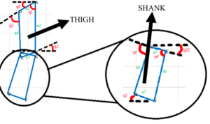
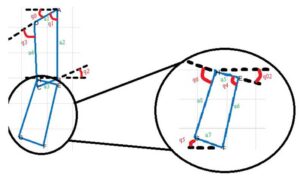
For the loop in thigh, the close loop equation is given by
a2*cos(q0+q1) + a2*sin(q0+q1) + a2*cos(q2) + a3*sin(q2) = a1*cos(q0) + a1*sin(q0) + a4*cos(q3+q0) + a4*sin(q3+q0)
q0, a1, a2, a3 and a4 are known and q1 is controlled by the servos which means q1 is independently changed by coding. q2 and q3 angles are the ones to be determined for every given q1 angle per unit time. At first the terms that are already known are taken to left side of the equation.
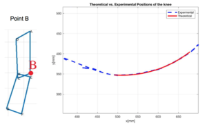
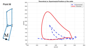
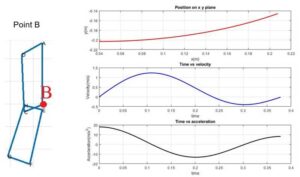
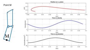
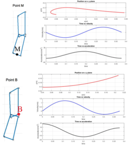
In matlab we solved these nonlinear equations using jacobian method. This method is a iterative method that solves these nonlinear equations based on iteration and error calculation. After solving equations we plotted them for two points that were important for our prıject. For our acceleration values we took time derivatives of the velocities int matlab again using an iterative derivative method. Our matlab code can be found in appendix.
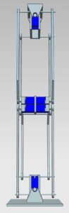
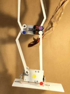
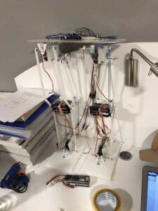
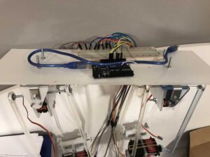
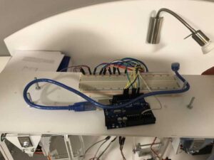
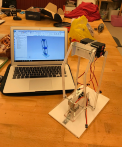
We first started by adjusting our Siemens NX CAD (computer aided design) parts for the laser cutter software in machine shop. We bought 70×70 cm^2 plexiglass with 5 mm thickness. After adjustments we laser cut our plexiglas parts at machine shop with the help of Muzaffer Bütün. We first wanted to have our robot to have two legs and a hip. Then we realized how difficult and expensive it would be to have two legs with motors(with enough torques). So we decided to see how it goes and make every decision on the fly. We decided to do the manufacturing step by step so if we make an error it doesn’t cost us all and we gradually increase the precision of our humanoid robot. So we cut the parts for one leg only and didn’t cut the parts for a second leg and hip. After cutting our leg we bought regular ball bearings, bolts and nuts, some from internet and other from nearby hardware stores.
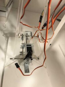
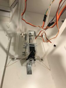
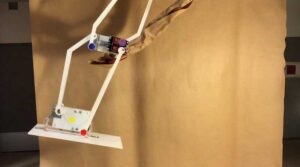
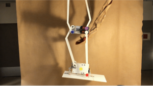
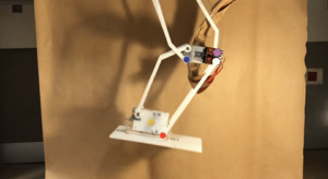
For the experimental setup we used one leg. We needed to stabilize the hip connection of the leg so we used a dog wrench and wooden, plexiglass parts. We stabilized the leg on a table and for the background we put a brown bag and taped it to the table and the ground. We put different colored stickers on the important points. Afterwards we filmed the motion and did our color tracking code.
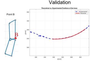
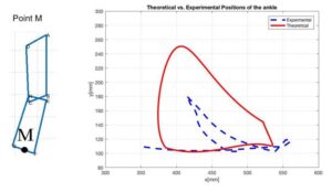
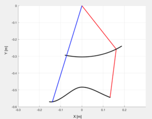
We can observe that the characteristics of the curves are same but the amplitude of the curves are different. Experimental curve has a much smaller amplitude and that is due to low torque servos that we used. Our servo motors even though we calculated them didn’t have enough torque and that was due to out lack of calculations of the swinging motion of the robot leg.