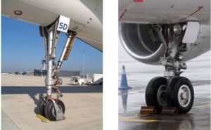
Landing gear of an aircraft is one of the vital parts in a well-functioning airplane. It is important in number of ways including the use during takeoff, landing, and at rest for supporting purposes. Throughout its history, landing gears saw many important developments that helped in many areas. Choosing the right landing gear on an aircraft is purely depended on the purpose of that aircraft. Usually, wheels are attached to the landing gear but for different purposes, it can also include skids, skis, floats, or a combination of these elements for different surfaces.
With the development of technology, we now have many different designs for retractable landing gears and our task was to design another. While designing our system, we considered all five requirements that were mentioned above and tried our best to achieve the best result in all of them. Further details can be found later in the report.

Meet Our Team

UFUK AKULKER
KUTAY GOZALAN
ANIL KEKLIKOGLU
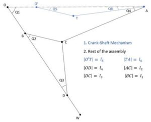
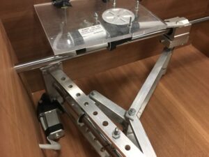
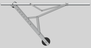
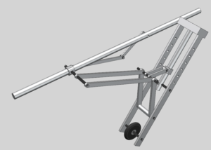
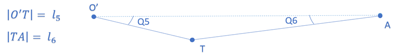
The primitive design of the project initially consisted of a three-bar mechanism. Then, responding to our TA’s request, the design was changed to a four-bar mechanism to achieve a more sophisticated design and possibly had more complex dynamics equations to solve. The final mechanism that is decided upon consists of seven rotational joints represented by points in Figure 1 and two slider motions at positions A and B. The mechanism is accepted as a four-bar mechanism since the two bars represented by O’T and AT are components of the crank-shaft mechanism actuated around O’, which is investigated and hence accepted as an individual mechanism that is separated from the rest of the assembly. The crank-shaft mechanism functions to attain the slider motion to the joint at the position A.
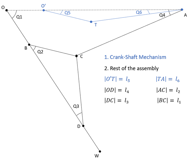
In order to investigate the dynamic behavior of the system it is decided to divide the system into two as the crank-shaft mechanism and the rest of the assembly. Because by doing so, potentially we would be able to reduce the system into a problem with known parameters of joint A, at any instant and without a crank-shaft mechanism. Relative motion analysis used below to solve the instantaneous position, velocity and acceleration of the joints.
After deriving the dynamic equations, we needed to make sure everything goes as planned and our system is correct. To do that, we implemented our equations to MATLAB and made a simulation of our design.
As discussed in above sections (especially in section 5) there are two mechanisms driving this system. One of them controls the angle in Point O, and the other controls Point A via a crankshaft mechanism mounted in point O’. So, we have two degrees of freedom in our system as there are two motors and two control points for each motor.
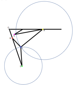
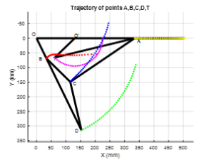
Figure 6.1: Solving method to find point C and B. Two circles that are centered at point A and point D, having radiuses of length |AC| and |DC| respectively.
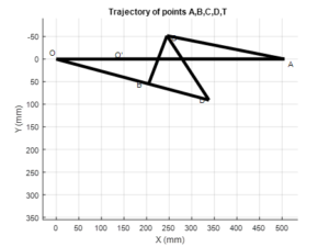
This simulation was satisfactory in all ways for us because all points reflected the realistic results that we were expecting. The method we used to simulate the motion was very rational and easy. We thought of the system as 4 bars that included |OA|, |AC|, |CD|, |DO|. We know the position of A (driven by a crankshaft), and point D (driven by the motor at point O). The lengths were also known for all bars, so we drew circles that centered at point A and point D, having radiuses of length |AC| and |CD|, respectively.
We chose geometrical way as we simulate the system because writing the code for geometric equations was easier and less time consuming. After the implementation, we found out that everything was working correctly if we do some assumptions on the system such as the relations between the angles. We were struggling with the geometric relations at the beginning, so just to see the system, we implemented these assumptions. These later got solved and no assumptions were made in the final simulation and every relation between the angles were found using conventional geometric methods.
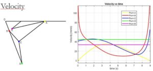
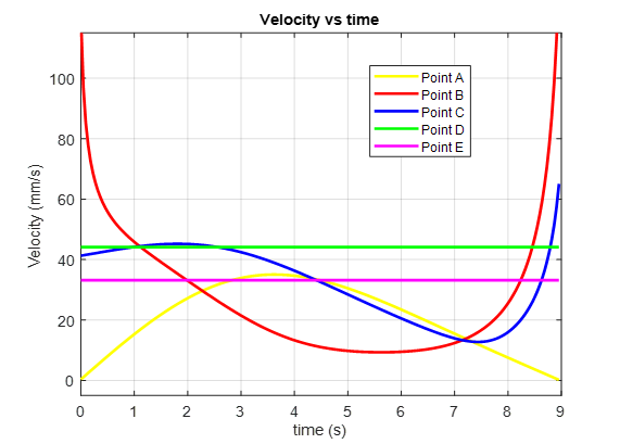
After having the positions, we were now ready to have the velocity and acceleration graphs. We can acquire velocity and acceleration graphs in two ways just like positions: 1- From dynamic equations that we derived or 2- taking the derivatives of position data using MATLAB’S diff() function, which calculates the differences between adjacent elements of positions along the position array (MathWorks).
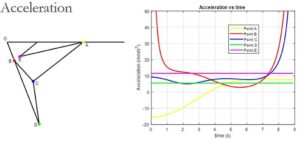
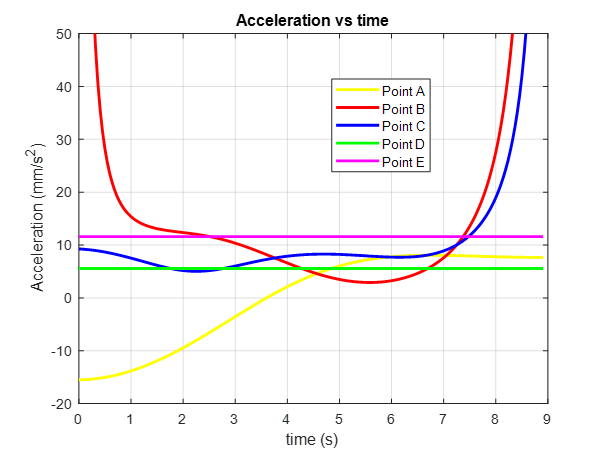
Acceleration graph is also fine, and we can understand that by looking at Points D and E again. Some may say that we must have zero acceleration because we know that Points D and E are making “uniform” circular motion but that is not necessarily true. While we have constant velocity, our point does “circular motion”, and that means that we would have 2 acceleration components, namely tangential and radial. The direction of both tangential and radial acceleration changes while moving, but radial is always normal, and tangential is always parallel to the velocity vector. Also, their magnitude is always the same and constant. Knowing these information, and looking at the graph, we can confirm that this graph is valid.
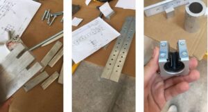
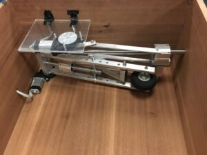
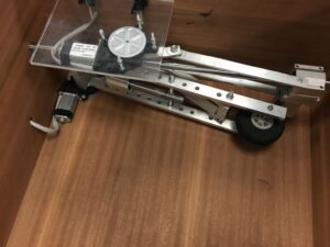
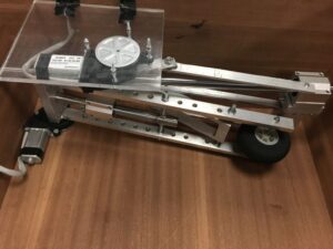
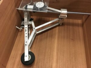
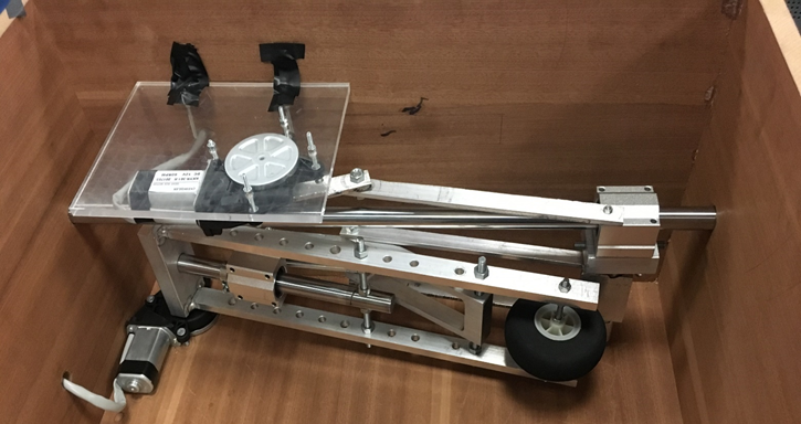
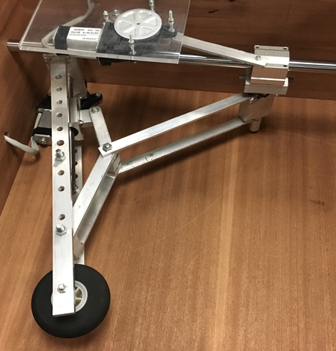
First, the material used for the assembly including the crank-shaft mechanism was aluminum. The material is selected to minimize the weight of the assembly which was calculated as 2.54 kilograms after manufacturing was completed.
After the material is selected, to start manufacturing technical drawings of the materials are printed and used to purchase chunks of aluminum. The dimensions of aluminum cut and purchased decided with respect to the dimensions in technical drawings.
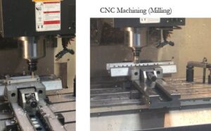
Then, for shaping the raw material, CNC Machinery and drilling mills are used. CNC Machinery was used to resize the material and cut the excess material and open grooves to minimize the weight according to the dimension given by the design. The drilling mill was used to open holes for the pins to enter.
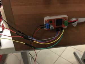
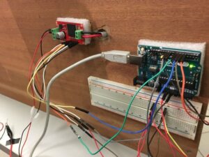
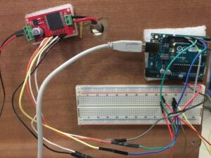
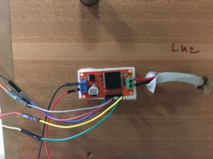
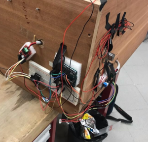
Electrical circuit designed and used in the system may also be investigated under manufacturing. For the circuit design, a breadboard, two direct-current motor drivers, two Arduino UNOs, a current amplifier and two high-torque, direct-current motors were used. The circuit is designed and controlled by our TA. Circuit design is presented below:
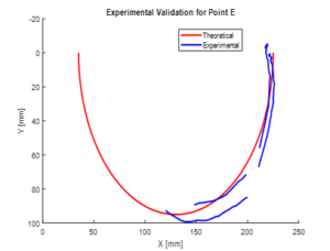
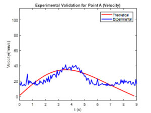
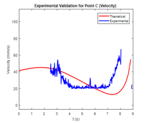
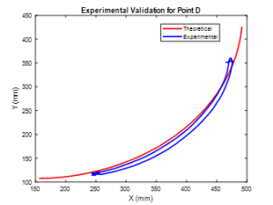
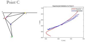
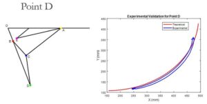
After manufacturing, we needed to make sure that our theoretical positions, velocities, and accelerations match with real values. To do that, we attached a yellow sticker to the points that we wanted to analyze, recorded a video of it, and sent it to MATLAB for color tracking. With this way, we obtained the real (experimental) positions for important points. After that, finding the velocity and accelerations of those points were found just by taking the derivate with MATLAB’s diff() function.
Although we wanted to have all the points for experimental validation, some limitations we had prevented us from collecting data. One of the major limitation was the blockage of view from our parts. We couldn’t attach stickers to some points due to them being at the rear of our parts. Graphs of our experimental validations for important points can be found below.