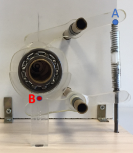
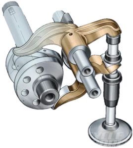
Desmodromic valve system is a form-closed valve cam train system. This mechanism, as opposed to the conventional valve system, does not contain any springs that are assigned to perform the valve closing operation. The lack of having any opposing spring force in the system has the benefit of ensuring not to lose any energy in the opening phase of the valves. The presence of a positive valve closer ensures the full sealing of the valves and prevents situations like valve float and follower jump. The duty of the only spring that is present in the mechanism is to ensure the constant contact of the rockers to the cams and has near to nothing effect on the energy consumption compared to the conventional valve systems.
The system has a set of cons along with its pros. For each valve there is an extra set of cam and rocker, which comes with a production cost. The maintenance of the system is harder than the conventional systems and it is argued that desmodromic valve cam trains experience more wearing than the conventional ones.
Due to safe and extremely good performance output along with high cost of production and maintenance, desmodromic valve system is mostly located as a prime and uncommon choice in the market. Many of the products utilizing the system are high performance, rare racing motorbikes or automobiles.
Meet Our Team
BERKE OZNALBANT
BURAK TOSUN
AHMET ACAR
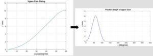
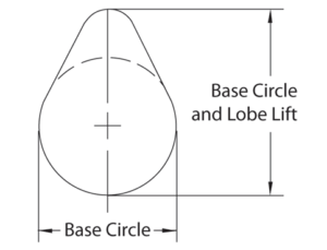
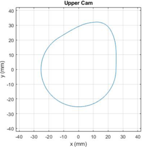
Base circle of a cam is the part of the cam function which does not give any lift output as seen on Figure 2. Since the displacement from the center of rotation is zero there is no rise. The radius of the base circle is often a concern of wearing, production cost and availability of space. In this project, since there are no limitations on wearing due to low rpm, no limitations on cost due to materials utilized and no limitations of space; radius of base circle is determined in the way that it is easiest to manufacture.
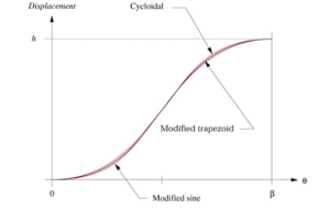
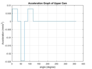
The fundamental law of cam design states that the displacement, velocity and acceleration functions must have no discontinuities. This leads to a condition known also as finite jerk. The cam functions we utilized for this project will be discussed in the Mechanism Design. Figure 3 below is showing an example set of three different functions’ displacement for first Beta degrees.
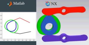
This projects design part started with matlab by creating relevant cam functions and deciding on the base circle radius. In order to forge an industry standard cam function the triple contour method is utilized. A matlab code is written which acquires knot points of four different functions with predetermined degrees and the desired lift from the user. Then the code gives out the final shape of the cam with the help of another block of code that is written, which takes the calculated cam function and the base circle radius as input. A further inquiry about the code is going to be held on Matlab Programming part. Then the shape of the cam is delivered to the NX, this will be discussed in the CAD Model Creation part.
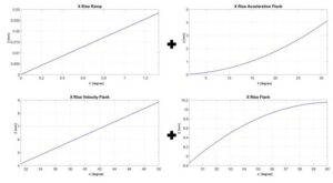
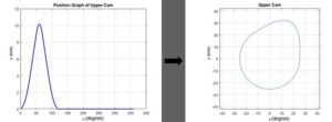
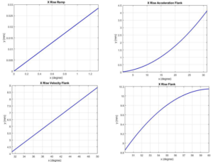
Triple contour method, which is a design method utilizes knowledge of spline functions, is employed in order to craft the desired cam profiles. Final displacement function which is achieved through triple contour method is a combination of nine different functions. Four of these functions are assigned to lift the follower and four others mission is to lower it. One remaining function is a constant function whose duty is to perform high or low dwells. Order of these functions from 0° to 360° for upper cam is X Rise Ramp, X Rise Acceleration Flank, X Rise Velocity Flank, X Rise Nose, X Fall Nose, X Fall Velocity Flank, X Fall Acceleration Flank, X Fall Ramp and X Low Dwell. The reason, this design procedure has the name “Triple Contour” is that, in order to lift or lower the rocker, three different functions are utilized. First and last functions, omitting the dwell part, which are named X Rise Ramp and X Fall Ramp are industry standard functions to have, therefore these two functions are not accepted as contours. Nine other functions for lower cam are crafted in the same manner.
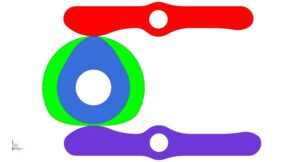
Four main CAD models are created for this project. They are categorized in two groups as cams and rockers. Cams are not directly created in NX. The shape of the cams are crafted in Matlab as it was mentioned in the Mechanical Design part and the shapes are transferred to the NX in order to create 3D CAD models. An array is created in MATLAB which contained data points of the coordinates of the shapes and these data points are saved to a text file. To NX, these points are imported and the spline command is used to connect the points.
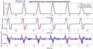
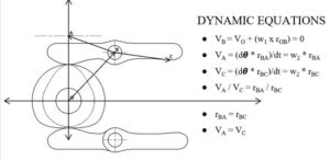
One dynamic equation is defined for the upper rocker arm. The upper rocker arm consists of two dynamic, rotating lines as it can be seen from figure below: AB and BC. Point A is selected as a critical point as it is the center of the arc that has been mentioned before in the Mechanical Design part. The contact point of the upper rocker and the upper cam is always along this arc. The center of the arc, which is point A, shares the same displacement values with the cam profiles displacement function. This deduction allows one to make experimental inquiry and validation under the lights of solved dynamic equations. While the experimental comparison will be held on Discussion of Theoretical and Experimental Results and Their Comparison part, solved dynamic equations of interest are below.

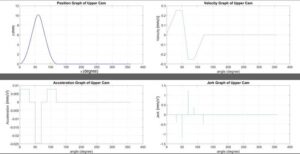
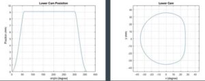
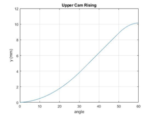
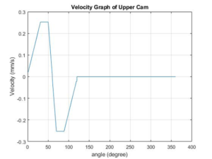
After deciding the functions’ degrees for the cam profiles, a matlab code system is written in a way that the derivatives of the functions are continuous. This code acquires four different knot points of the four different functions those, at the end, cumulatively form a rise function. Than, since a symmetric profile is demanded, a symmetric fall function is crafted. The amount of low and high dwell were predetermined. The demanded amount of lift is also obtained from the user. MATLAB is used for creating the cam profiles instead of Siemens NX as the complete precision is needed. With the help of the code, two different cam profiles are acquired, upper and lower cam, from different function sets. Since the position function of every point on the cam profile is known, taking derivatives of these position vectors give the velocity, acceleration and jerk graphs. These graphs are crucial for this project since the aim was to obtain industry standard cam profiles. In order to achieve this goal one had to comply with the fundamental law of cam design. It is confirmed that the velocity and acceleration graphs are continuous by drawing their graph with respect to time.
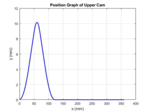
The output of the functions are the displacement of each point from the base circle to the outer border with respect to the center point. We wrote another code block which takes the output from these functions and creates the cam profile accordingly with precision.
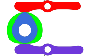
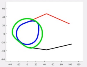
It was crucial to animate the motion in MATLAB to get the theoretical data points, which are belong to rockers’ displacement values, to compare the theoretical and experimental data. Cam profiles are drawn by the code and the rockers are illustrated as lines for the sake of simplicity. Position of the center of rockers and cams are decided in NX. After drawing and placing the parts, constant angular velocity is given to the cams, the rockers had moved accordingly. Finally, theoretical data points are taken from the MATLAB animation and later added into the experimental data to compare.
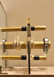
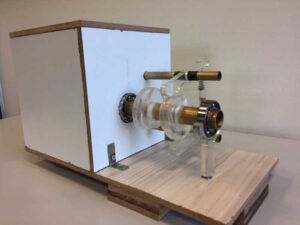
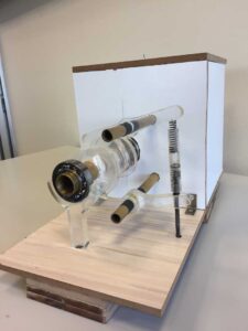
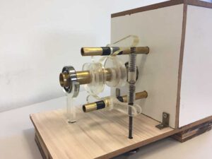
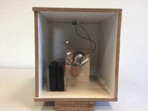
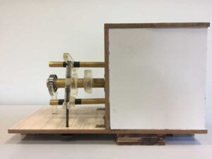
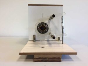
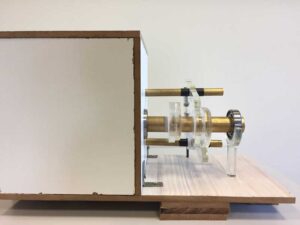
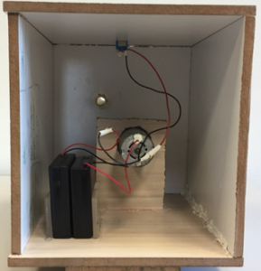
The calculations and assumptions gave clue about the required general properties about motor and a 12 volt, 0.75 ampere and 75 rpm reducer dc motor which has 18 kgf.s strain torque is chosen. Two 6005 ball bearing, in order to reduce friction of the main shaft, are utilized. For all system; three shafts, one for main and two for rockers, is needed. The first choice was aluminum but the appropriate shaft was not found. The next choice is brass as this material is cheaper and stronger than aluminum and there are no significant weight differences in between. Bigger brass shaft has 25 mm and the other two has 12 mm diameter. Bigger shaft is connected to the platform with two bearings but the other two shafts are fixed. MDF choice is made for the platform and the section where the motor and batteries are located is covered. The back side is left open for possible adjustment and interventions. In the back side two batteries, motor and motor shaft connection device are placed, also two rocker shafts are fixed to MDF. For fixing process, after some research, two different adhesives are found to be appropriate. In order to fix metal to metal, Loctite is applied. Loctite is a very robust adhesive but it is not appropriate to fix different kinds of materials. Therefore, another strong adhesive with activator is utilized in such situations. Cams and rockers are produced in the Laser Lab in Koç University. Total of four cams are manufactured. Two of them are counterweights which are directed to exact opposite sides to the operating cams . The purpose of the counterweights is to bring the center of gravity to the center axis of the shaft thus preventing the jerky motion, which is a critical issue in the industry but for this project is not crucial due to low rpm value. Also, it was necessary to create a perfect fit between the motor and the shaft.

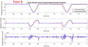
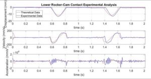
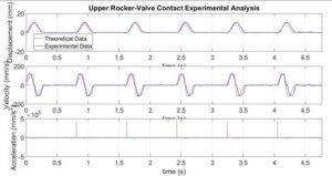
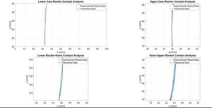
As suggested, markers are placed on the critical points of the upper and lower rockers and MATLAB image tracking is used on these points. A wooden piece with one centimeter margins is placed next to the system in order to be used as a reference frame. Then the camera is put in a fixed position and the motion is recorded. Several changes are made in the MATLAB image tracking code to integrate it with the project. Below, it can be seen that displacement values for point B are equal to the displacement values of the calculated cam profile. This can be stated as a validation to the first assumption while deriving the dynamic equations, which states that the center of the circle follows the same displacement functions as the profile. Although point B is not the center of the arc, this point is connected to the center point with a non-dynamic constant link; so this point is going to have same displacement figures. Further comparison between the experimental measured data and the theoretical data derived for point A, with the knowledge of dynamic equations, is made in figure below. As it can be seen, theoretical and experimental data are consisted although the measurement method was not so accurate. The dynamic equations are validated. The jump in the theoretical value for acceleration graph is due to programming error and should not be taken into consideration.