Here we begin the journey that is graphing with R. The ability to make beautiful and compelling graphs quickly was what drew me into using R in the first place. Later, I began to use graphing packages like ggplot2 and ggvis and quickly found that making high quality and publishable plots is easy. Perhaps one of the most exciting (and new) features of R is the introduction of packages like shiny which allow for direct translation of R code into javascript code. Later we will be exploring some of these exciting uses of R. Particularly, we will focus on how to make an interactive report where someone can drag a slider bar around to adjust aspects of your graph. A sure sign that you are bound for promotion!
Lesson 2: Graphing with Base-R
Scott Withrow
June 29, 2015
Graphing in R is very powerful. Think of graphing in R as a construction project. We start by laying down a foundation (specifying the data), then we build the framework (specifying the axes, labeling, titling, etc.), then we fill in the rest of the structure with the walls and details (specifying the statistics that are displayed in the graph). Base-R has a large suite of tools for graphing and does a commendable job quickly plotting what researchers need to see. The tools exist to build a plot that you desire but many turn to packages for true graphing freedom. The most propular packages are lattice and ggplot2 with the sucessor to ggplot2, ggvis, gaining in popularity. We will later be covering ggplot2 since it is more refined and less subject to change than ggvis.
We will work with one of the R learning dataframes today. The data was extracted from the 1974 Motor Trend US magazine, and comprises fuel consumption and 10 aspects of automobile design and performance for 32 automobiles (1973-74 models)
head(mtcars)## mpg cyl disp hp drat wt qsec vs am gear carb
## Mazda RX4 21.0 6 160 110 3.90 2.620 16.46 0 1 4 4
## Mazda RX4 Wag 21.0 6 160 110 3.90 2.875 17.02 0 1 4 4
## Datsun 710 22.8 4 108 93 3.85 2.320 18.61 1 1 4 1
## Hornet 4 Drive 21.4 6 258 110 3.08 3.215 19.44 1 0 3 1
## Hornet Sportabout 18.7 8 360 175 3.15 3.440 17.02 0 0 3 2
## Valiant 18.1 6 225 105 2.76 3.460 20.22 1 0 3 1summary(mtcars)## mpg cyl disp hp
## Min. :10.40 Min. :4.000 Min. : 71.1 Min. : 52.0
## 1st Qu.:15.43 1st Qu.:4.000 1st Qu.:120.8 1st Qu.: 96.5
## Median :19.20 Median :6.000 Median :196.3 Median :123.0
## Mean :20.09 Mean :6.188 Mean :230.7 Mean :146.7
## 3rd Qu.:22.80 3rd Qu.:8.000 3rd Qu.:326.0 3rd Qu.:180.0
## Max. :33.90 Max. :8.000 Max. :472.0 Max. :335.0
## drat wt qsec vs
## Min. :2.760 Min. :1.513 Min. :14.50 Min. :0.0000
## 1st Qu.:3.080 1st Qu.:2.581 1st Qu.:16.89 1st Qu.:0.0000
## Median :3.695 Median :3.325 Median :17.71 Median :0.0000
## Mean :3.597 Mean :3.217 Mean :17.85 Mean :0.4375
## 3rd Qu.:3.920 3rd Qu.:3.610 3rd Qu.:18.90 3rd Qu.:1.0000
## Max. :4.930 Max. :5.424 Max. :22.90 Max. :1.0000
## am gear carb
## Min. :0.0000 Min. :3.000 Min. :1.000
## 1st Qu.:0.0000 1st Qu.:3.000 1st Qu.:2.000
## Median :0.0000 Median :4.000 Median :2.000
## Mean :0.4062 Mean :3.688 Mean :2.812
## 3rd Qu.:1.0000 3rd Qu.:4.000 3rd Qu.:4.000
## Max. :1.0000 Max. :5.000 Max. :8.000str(mtcars)## 'data.frame': 32 obs. of 11 variables:
## $ mpg : num 21 21 22.8 21.4 18.7 18.1 14.3 24.4 22.8 19.2 ...
## $ cyl : num 6 6 4 6 8 6 8 4 4 6 ...
## $ disp: num 160 160 108 258 360 ...
## $ hp : num 110 110 93 110 175 105 245 62 95 123 ...
## $ drat: num 3.9 3.9 3.85 3.08 3.15 2.76 3.21 3.69 3.92 3.92 ...
## $ wt : num 2.62 2.88 2.32 3.21 3.44 ...
## $ qsec: num 16.5 17 18.6 19.4 17 ...
## $ vs : num 0 0 1 1 0 1 0 1 1 1 ...
## $ am : num 1 1 1 0 0 0 0 0 0 0 ...
## $ gear: num 4 4 4 3 3 3 3 4 4 4 ...
## $ carb: num 4 4 1 1 2 1 4 2 2 4 ...help(mtcars) for more info on the dataset.
This is an American dataset so we can convert to metric for measurements that make sense. Like we did in lesson 1 we use within to state which dataframe to use (in this case mtcars). Then we use a curly bracket to frame what we want to manipulate. The curly brackets help keep the syntax organized. At the end we assign the data back to the mtcars datafame with a right facing arrow.
within(mtcars, {
  kpl <- mpg * 0.425
  wt.mt <- wt * 0.454
  disp.c <- disp * 2.54
}) -> mtcars
The Most Basic Graph
First we lay the foundation
Graph weight by kilometers per liter.
We are using the mtcars dataframe and some variables that are in that dataframe. Like in lesson 1 we need to tell R what dataframe the variables are in. We do that by using the $. mtcars is the data and WITHIN ($) that data is the variable wt.mt.
Then we overlay that foundation with a least squares line.
abline = straight line graphic
lm = linear model
~ is the by command here we are saying graph kpl by wt.ml
plot(mtcars$wt.mt, mtcars$kpl)
abline(lm(mtcars$kpl ~ mtcars$wt.mt))
title("Regression of Kilometers per Liter on Weight in Metric Tons")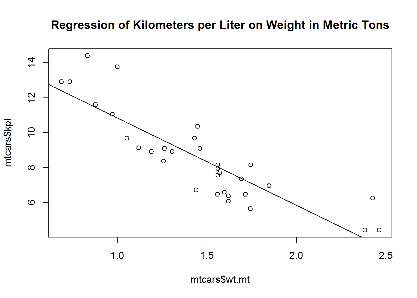
Now let’s put some strucural components in place
Saving a Graph to the Hard Drive
I am too lazy to make a folder so let’s have R do it for us.
dir.create("E:/Rcourse/L2", showWarnings = FALSE)Make that new folder the working directory.
setwd("E:/Rcourse/L2")Let’s take the commands above and create a file instead of displaying.
First we need to tell what engine to use. I prefer png since it’s a good mix of compression and quality. You can specify pdf or tiff for good lossless saves, jpg for small and low quality, or bmp, xfig, and postscript for embedding or modifications. Just be sure that whatever engine you specify you also specify a file extention that matches.
This will start a graphical device (dev) which saves console output to that device until it ends with dev.off(). You could use this to capture table output or anything else you like.
png("graph1.png")
plot(mtcars$wt.mt, mtcars$kpl)
abline(lm(mtcars$kpl ~ mtcars$wt.mt))
title("Regression of Kilometers per Liter on Weight in Metric Tons")
dev.off()
## png
## 2Notice nothing is generated in the plot window.
You can specify the size of the graph in the dev with width, height, and units. You can also specify plotted point size with pointsize, background with bg, resolution in ppi with res, and depending on the file type some measure of quality or compression type. See ?png or ?pdf for more information.
png("graph2.png", width = 1000, height = 806, units = "px", res = 150)
plot(mtcars$wt.mt, mtcars$kpl)
abline(lm(mtcars$kpl ~ mtcars$wt.mt))
title("Regression of Kilometers per Liter on Weight in Metric Tons")
dev.off()
## png
## 2Here we are specifying a graph that is 1000 by 806 pixels and adjusting res so the graph isn’t tiny at that size
If you have been saving images and suddenly your commands don’t seem to be doing anything anymore it’s probably because a dev is still running. You can simply run dev.off() until R prints null device 1 or gives the error “cannot shut down device 1”
R studio also support saving a graph through the point and click menus. Check the export box and modify settings accordingly.
Making Graphs Pretty and Functional
R controls graph displays with graphical parameters or par(). They function as par(optionname=VALUE, optionname=VALUE)
par(no.readonly=TRUE) #These are all the parameters you can manipulate.## $xlog
## [1] FALSE
##
## $ylog
## [1] FALSE
##
## $adj
## [1] 0.5
##
## $ann
## [1] TRUE
##
## $ask
## [1] FALSE
##
## $bg
## [1] "white"
##
## $bty
## [1] "o"
##
## $cex
## [1] 1
##
## $cex.axis
## [1] 1
##
## $cex.lab
## [1] 1
##
## $cex.main
## [1] 1.2
##
## $cex.sub
## [1] 1
##
## $col
## [1] "black"
##
## $col.axis
## [1] "black"
##
## $col.lab
## [1] "black"
##
## $col.main
## [1] "black"
##
## $col.sub
## [1] "black"
##
## $crt
## [1] 0
##
## $err
## [1] 0
##
## $family
## [1] ""
##
## $fg
## [1] "black"
##
## $fig
## [1] 0 1 0 1
##
## $fin
## [1] 6.999999 4.999999
##
## $font
## [1] 1
##
## $font.axis
## [1] 1
##
## $font.lab
## [1] 1
##
## $font.main
## [1] 2
##
## $font.sub
## [1] 1
##
## $lab
## [1] 5 5 7
##
## $las
## [1] 0
##
## $lend
## [1] "round"
##
## $lheight
## [1] 1
##
## $ljoin
## [1] "round"
##
## $lmitre
## [1] 10
##
## $lty
## [1] "solid"
##
## $lwd
## [1] 1
##
## $mai
## [1] 1.02 0.82 0.82 0.42
##
## $mar
## [1] 5.1 4.1 4.1 2.1
##
## $mex
## [1] 1
##
## $mfcol
## [1] 1 1
##
## $mfg
## [1] 1 1 1 1
##
## $mfrow
## [1] 1 1
##
## $mgp
## [1] 3 1 0
##
## $mkh
## [1] 0.001
##
## $new
## [1] FALSE
##
## $oma
## [1] 0 0 0 0
##
## $omd
## [1] 0 1 0 1
##
## $omi
## [1] 0 0 0 0
##
## $pch
## [1] 1
##
## $pin
## [1] 5.759999 3.159999
##
## $plt
## [1] 0.1171429 0.9400000 0.2040000 0.8360000
##
## $ps
## [1] 12
##
## $pty
## [1] "m"
##
## $smo
## [1] 1
##
## $srt
## [1] 0
##
## $tck
## [1] NA
##
## $tcl
## [1] -0.5
##
## $usr
## [1] 0 1 0 1
##
## $xaxp
## [1] 0 1 5
##
## $xaxs
## [1] "r"
##
## $xaxt
## [1] "s"
##
## $xpd
## [1] FALSE
##
## $yaxp
## [1] 0 1 5
##
## $yaxs
## [1] "r"
##
## $yaxt
## [1] "s"
##
## $ylbias
## [1] 0.2Lets change the shape of the dot to a triangle and the line to a dashed one. The first step is to save the default parameters. It is not essential that you do so but it helps reset things if you mess up and don’t remember what you did or how to fix the mistake.
defaultpar <- par(no.readonly=TRUE)

par(lty=2, pch=17)
plot(mtcars$wt.mt, mtcars$kpl)
abline(lm(mtcars$kpl ~ mtcars$wt.mt))
title("Regression of Kilometers per Liter on Weight in Metric Tons")
par(defaultpar)In RStudio you can also reset your parameters to the default by clicking Clear All in the plots window.
Common parameters
lty = line type
pch = plotted point type
cex = symbol size
lwd = line width
How can I find more? ?par or help(“par”)
Most plot functions allow you to specify everything inline. This tends to be how I modify plot options. It only lasts for one plot but in my experience I am seldom changing every point in dozens of graphs to warrent using global pars.
plot(mtcars$wt.mt, mtcars$kpl, lty=2, pch=17,
     abline(lm(mtcars$kpl ~ mtcars$wt.mt)),
     main="Regression of Kilometers per Liter on Weight in Metric Tons")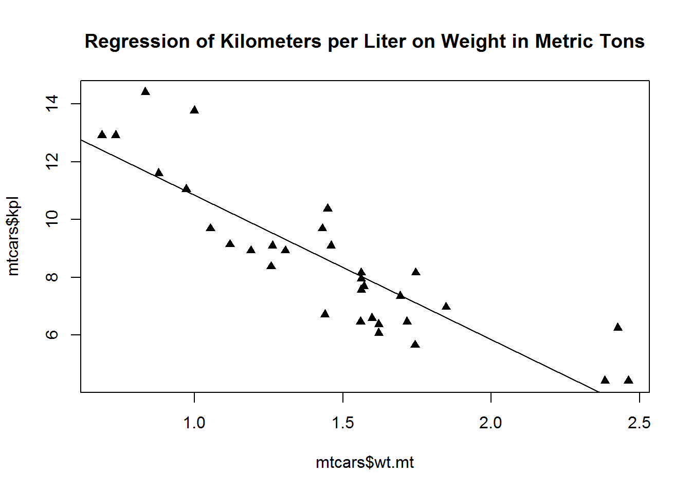
Like with the lm we can specify some graphs to use the by.
The form is Y ~by~ X
boxplot(mtcars$kpl ~ mtcars$gear,
        main = "Boxplot of Kilometers per Liter by Number of Gears")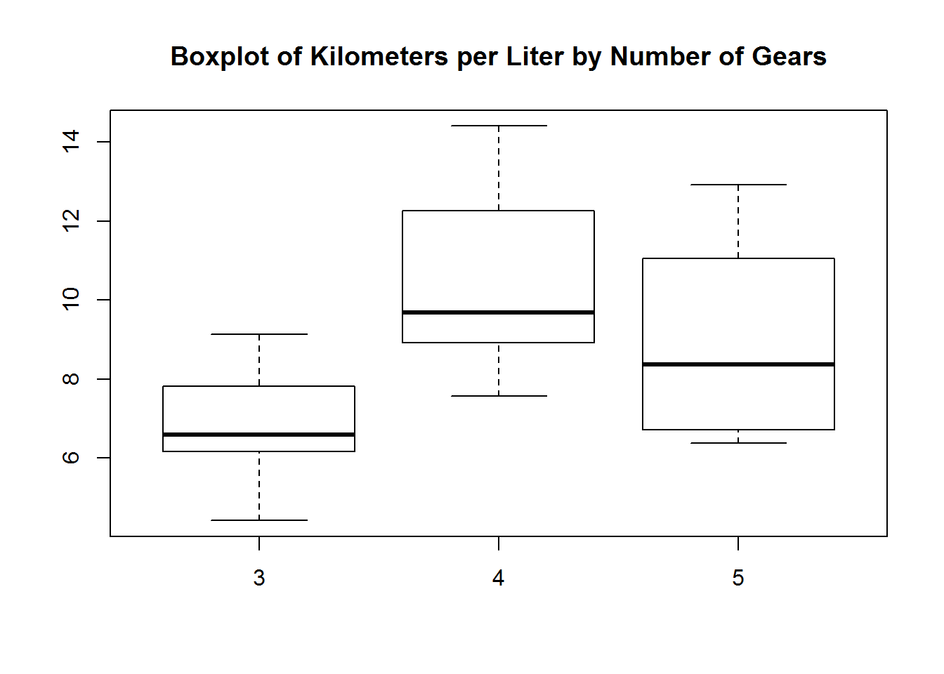
Coloring a graph.
Everything can be colored. col = plot color, col.axis = axis color, col.lab = labels color, col.main = title color, col.sub = subtitle color, fg = foreground color, and bg = background color. Color can be specified many ways:
col = 1 | Specified by order in R dataframe
col = “white” | Specified by name
col = #FFFFFF | Specified by hexadecimal
col = rgb(1,1,1) | Specified by RGB index
col = hsv(0,0,1) | Specified by HSV index
colors() #all the names and index numbers for the R colors## [1] "white" "aliceblue" "antiquewhite"
## [4] "antiquewhite1" "antiquewhite2" "antiquewhite3"
## [7] "antiquewhite4" "aquamarine" "aquamarine1"
## [10] "aquamarine2" "aquamarine3" "aquamarine4"
## [13] "azure" "azure1" "azure2"
## [16] "azure3" "azure4" "beige"
## [19] "bisque" "bisque1" "bisque2"
## [22] "bisque3" "bisque4" "black"
## [25] "blanchedalmond" "blue" "blue1"
## [28] "blue2" "blue3" "blue4"
## [31] "blueviolet" "brown" "brown1"
## [34] "brown2" "brown3" "brown4"
## [37] "burlywood" "burlywood1" "burlywood2"
## [40] "burlywood3" "burlywood4" "cadetblue"
## [43] "cadetblue1" "cadetblue2" "cadetblue3"
## [46] "cadetblue4" "chartreuse" "chartreuse1"
## [49] "chartreuse2" "chartreuse3" "chartreuse4"
## [52] "chocolate" "chocolate1" "chocolate2"
## [55] "chocolate3" "chocolate4" "coral"
## [58] "coral1" "coral2" "coral3"
## [61] "coral4" "cornflowerblue" "cornsilk"
## [64] "cornsilk1" "cornsilk2" "cornsilk3"
## [67] "cornsilk4" "cyan" "cyan1"
## [70] "cyan2" "cyan3" "cyan4"
## [73] "darkblue" "darkcyan" "darkgoldenrod"
## [76] "darkgoldenrod1" "darkgoldenrod2" "darkgoldenrod3"
## [79] "darkgoldenrod4" "darkgray" "darkgreen"
## [82] "darkgrey" "darkkhaki" "darkmagenta"
## [85] "darkolivegreen" "darkolivegreen1" "darkolivegreen2"
## [88] "darkolivegreen3" "darkolivegreen4" "darkorange"
## [91] "darkorange1" "darkorange2" "darkorange3"
## [94] "darkorange4" "darkorchid" "darkorchid1"
## [97] "darkorchid2" "darkorchid3" "darkorchid4"
## [100] "darkred" "darksalmon" "darkseagreen"
## [103] "darkseagreen1" "darkseagreen2" "darkseagreen3"
## [106] "darkseagreen4" "darkslateblue" "darkslategray"
## [109] "darkslategray1" "darkslategray2" "darkslategray3"
## [112] "darkslategray4" "darkslategrey" "darkturquoise"
## [115] "darkviolet" "deeppink" "deeppink1"
## [118] "deeppink2" "deeppink3" "deeppink4"
## [121] "deepskyblue" "deepskyblue1" "deepskyblue2"
## [124] "deepskyblue3" "deepskyblue4" "dimgray"
## [127] "dimgrey" "dodgerblue" "dodgerblue1"
## [130] "dodgerblue2" "dodgerblue3" "dodgerblue4"
## [133] "firebrick" "firebrick1" "firebrick2"
## [136] "firebrick3" "firebrick4" "floralwhite"
## [139] "forestgreen" "gainsboro" "ghostwhite"
## [142] "gold" "gold1" "gold2"
## [145] "gold3" "gold4" "goldenrod"
## [148] "goldenrod1" "goldenrod2" "goldenrod3"
## [151] "goldenrod4" "gray" "gray0"
## [154] "gray1" "gray2" "gray3"
## [157] "gray4" "gray5" "gray6"
## [160] "gray7" "gray8" "gray9"
## [163] "gray10" "gray11" "gray12"
## [166] "gray13" "gray14" "gray15"
## [169] "gray16" "gray17" "gray18"
## [172] "gray19" "gray20" "gray21"
## [175] "gray22" "gray23" "gray24"
## [178] "gray25" "gray26" "gray27"
## [181] "gray28" "gray29" "gray30"
## [184] "gray31" "gray32" "gray33"
## [187] "gray34" "gray35" "gray36"
## [190] "gray37" "gray38" "gray39"
## [193] "gray40" "gray41" "gray42"
## [196] "gray43" "gray44" "gray45"
## [199] "gray46" "gray47" "gray48"
## [202] "gray49" "gray50" "gray51"
## [205] "gray52" "gray53" "gray54"
## [208] "gray55" "gray56" "gray57"
## [211] "gray58" "gray59" "gray60"
## [214] "gray61" "gray62" "gray63"
## [217] "gray64" "gray65" "gray66"
## [220] "gray67" "gray68" "gray69"
## [223] "gray70" "gray71" "gray72"
## [226] "gray73" "gray74" "gray75"
## [229] "gray76" "gray77" "gray78"
## [232] "gray79" "gray80" "gray81"
## [235] "gray82" "gray83" "gray84"
## [238] "gray85" "gray86" "gray87"
## [241] "gray88" "gray89" "gray90"
## [244] "gray91" "gray92" "gray93"
## [247] "gray94" "gray95" "gray96"
## [250] "gray97" "gray98" "gray99"
## [253] "gray100" "green" "green1"
## [256] "green2" "green3" "green4"
## [259] "greenyellow" "grey" "grey0"
## [262] "grey1" "grey2" "grey3"
## [265] "grey4" "grey5" "grey6"
## [268] "grey7" "grey8" "grey9"
## [271] "grey10" "grey11" "grey12"
## [274] "grey13" "grey14" "grey15"
## [277] "grey16" "grey17" "grey18"
## [280] "grey19" "grey20" "grey21"
## [283] "grey22" "grey23" "grey24"
## [286] "grey25" "grey26" "grey27"
## [289] "grey28" "grey29" "grey30"
## [292] "grey31" "grey32" "grey33"
## [295] "grey34" "grey35" "grey36"
## [298] "grey37" "grey38" "grey39"
## [301] "grey40" "grey41" "grey42"
## [304] "grey43" "grey44" "grey45"
## [307] "grey46" "grey47" "grey48"
## [310] "grey49" "grey50" "grey51"
## [313] "grey52" "grey53" "grey54"
## [316] "grey55" "grey56" "grey57"
## [319] "grey58" "grey59" "grey60"
## [322] "grey61" "grey62" "grey63"
## [325] "grey64" "grey65" "grey66"
## [328] "grey67" "grey68" "grey69"
## [331] "grey70" "grey71" "grey72"
## [334] "grey73" "grey74" "grey75"
## [337] "grey76" "grey77" "grey78"
## [340] "grey79" "grey80" "grey81"
## [343] "grey82" "grey83" "grey84"
## [346] "grey85" "grey86" "grey87"
## [349] "grey88" "grey89" "grey90"
## [352] "grey91" "grey92" "grey93"
## [355] "grey94" "grey95" "grey96"
## [358] "grey97" "grey98" "grey99"
## [361] "grey100" "honeydew" "honeydew1"
## [364] "honeydew2" "honeydew3" "honeydew4"
## [367] "hotpink" "hotpink1" "hotpink2"
## [370] "hotpink3" "hotpink4" "indianred"
## [373] "indianred1" "indianred2" "indianred3"
## [376] "indianred4" "ivory" "ivory1"
## [379] "ivory2" "ivory3" "ivory4"
## [382] "khaki" "khaki1" "khaki2"
## [385] "khaki3" "khaki4" "lavender"
## [388] "lavenderblush" "lavenderblush1" "lavenderblush2"
## [391] "lavenderblush3" "lavenderblush4" "lawngreen"
## [394] "lemonchiffon" "lemonchiffon1" "lemonchiffon2"
## [397] "lemonchiffon3" "lemonchiffon4" "lightblue"
## [400] "lightblue1" "lightblue2" "lightblue3"
## [403] "lightblue4" "lightcoral" "lightcyan"
## [406] "lightcyan1" "lightcyan2" "lightcyan3"
## [409] "lightcyan4" "lightgoldenrod" "lightgoldenrod1"
## [412] "lightgoldenrod2" "lightgoldenrod3" "lightgoldenrod4"
## [415] "lightgoldenrodyellow" "lightgray" "lightgreen"
## [418] "lightgrey" "lightpink" "lightpink1"
## [421] "lightpink2" "lightpink3" "lightpink4"
## [424] "lightsalmon" "lightsalmon1" "lightsalmon2"
## [427] "lightsalmon3" "lightsalmon4" "lightseagreen"
## [430] "lightskyblue" "lightskyblue1" "lightskyblue2"
## [433] "lightskyblue3" "lightskyblue4" "lightslateblue"
## [436] "lightslategray" "lightslategrey" "lightsteelblue"
## [439] "lightsteelblue1" "lightsteelblue2" "lightsteelblue3"
## [442] "lightsteelblue4" "lightyellow" "lightyellow1"
## [445] "lightyellow2" "lightyellow3" "lightyellow4"
## [448] "limegreen" "linen" "magenta"
## [451] "magenta1" "magenta2" "magenta3"
## [454] "magenta4" "maroon" "maroon1"
## [457] "maroon2" "maroon3" "maroon4"
## [460] "mediumaquamarine" "mediumblue" "mediumorchid"
## [463] "mediumorchid1" "mediumorchid2" "mediumorchid3"
## [466] "mediumorchid4" "mediumpurple" "mediumpurple1"
## [469] "mediumpurple2" "mediumpurple3" "mediumpurple4"
## [472] "mediumseagreen" "mediumslateblue" "mediumspringgreen"
## [475] "mediumturquoise" "mediumvioletred" "midnightblue"
## [478] "mintcream" "mistyrose" "mistyrose1"
## [481] "mistyrose2" "mistyrose3" "mistyrose4"
## [484] "moccasin" "navajowhite" "navajowhite1"
## [487] "navajowhite2" "navajowhite3" "navajowhite4"
## [490] "navy" "navyblue" "oldlace"
## [493] "olivedrab" "olivedrab1" "olivedrab2"
## [496] "olivedrab3" "olivedrab4" "orange"
## [499] "orange1" "orange2" "orange3"
## [502] "orange4" "orangered" "orangered1"
## [505] "orangered2" "orangered3" "orangered4"
## [508] "orchid" "orchid1" "orchid2"
## [511] "orchid3" "orchid4" "palegoldenrod"
## [514] "palegreen" "palegreen1" "palegreen2"
## [517] "palegreen3" "palegreen4" "paleturquoise"
## [520] "paleturquoise1" "paleturquoise2" "paleturquoise3"
## [523] "paleturquoise4" "palevioletred" "palevioletred1"
## [526] "palevioletred2" "palevioletred3" "palevioletred4"
## [529] "papayawhip" "peachpuff" "peachpuff1"
## [532] "peachpuff2" "peachpuff3" "peachpuff4"
## [535] "peru" "pink" "pink1"
## [538] "pink2" "pink3" "pink4"
## [541] "plum" "plum1" "plum2"
## [544] "plum3" "plum4" "powderblue"
## [547] "purple" "purple1" "purple2"
## [550] "purple3" "purple4" "red"
## [553] "red1" "red2" "red3"
## [556] "red4" "rosybrown" "rosybrown1"
## [559] "rosybrown2" "rosybrown3" "rosybrown4"
## [562] "royalblue" "royalblue1" "royalblue2"
## [565] "royalblue3" "royalblue4" "saddlebrown"
## [568] "salmon" "salmon1" "salmon2"
## [571] "salmon3" "salmon4" "sandybrown"
## [574] "seagreen" "seagreen1" "seagreen2"
## [577] "seagreen3" "seagreen4" "seashell"
## [580] "seashell1" "seashell2" "seashell3"
## [583] "seashell4" "sienna" "sienna1"
## [586] "sienna2" "sienna3" "sienna4"
## [589] "skyblue" "skyblue1" "skyblue2"
## [592] "skyblue3" "skyblue4" "slateblue"
## [595] "slateblue1" "slateblue2" "slateblue3"
## [598] "slateblue4" "slategray" "slategray1"
## [601] "slategray2" "slategray3" "slategray4"
## [604] "slategrey" "snow" "snow1"
## [607] "snow2" "snow3" "snow4"
## [610] "springgreen" "springgreen1" "springgreen2"
## [613] "springgreen3" "springgreen4" "steelblue"
## [616] "steelblue1" "steelblue2" "steelblue3"
## [619] "steelblue4" "tan" "tan1"
## [622] "tan2" "tan3" "tan4"
## [625] "thistle" "thistle1" "thistle2"
## [628] "thistle3" "thistle4" "tomato"
## [631] "tomato1" "tomato2" "tomato3"
## [634] "tomato4" "turquoise" "turquoise1"
## [637] "turquoise2" "turquoise3" "turquoise4"
## [640] "violet" "violetred" "violetred1"
## [643] "violetred2" "violetred3" "violetred4"
## [646] "wheat" "wheat1" "wheat2"
## [649] "wheat3" "wheat4" "whitesmoke"
## [652] "yellow" "yellow1" "yellow2"
## [655] "yellow3" "yellow4" "yellowgreen"You can also use this PDF
http://research.stowers-institute.org/efg/R/Color/Chart/ColorChart.pdf from
Earl F. Glynn’s page on Stowers Institute for Medical Research.
R also features a variety of premade pallets
For example,
Rainbow
N <- 10
Color <- rainbow(N)
pie(rep(1,N), col=Color)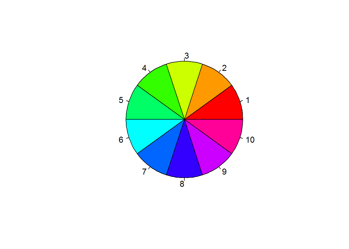
Gray
Color <- gray(0:N/N)
pie(rep(1,N), col=Color)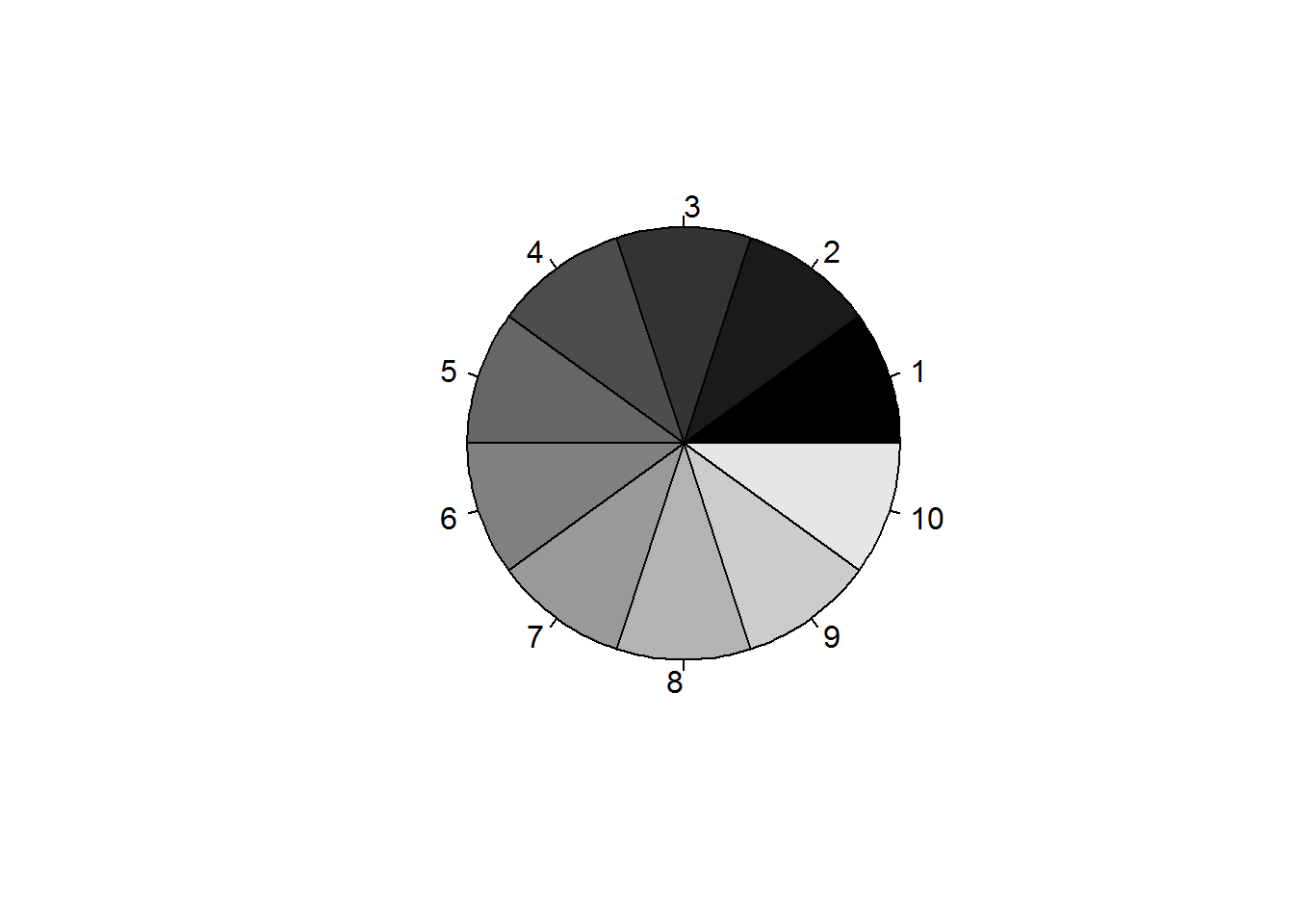
Heat
Color <- heat.colors(N)
pie(rep(1,N), col=Color)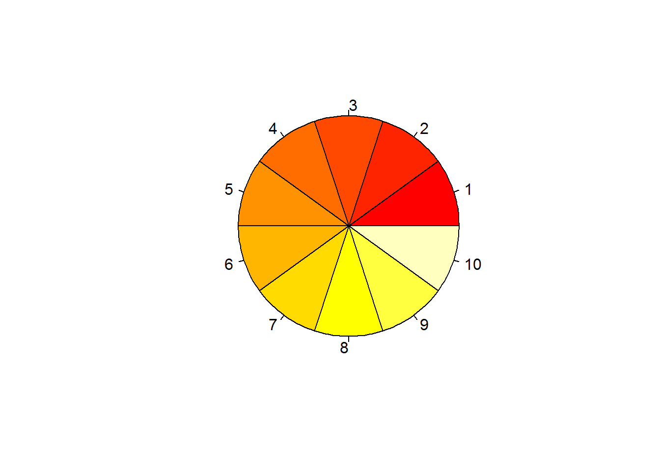
Topographic
Color <- topo.colors(N)
pie(rep(1,N), col=Color)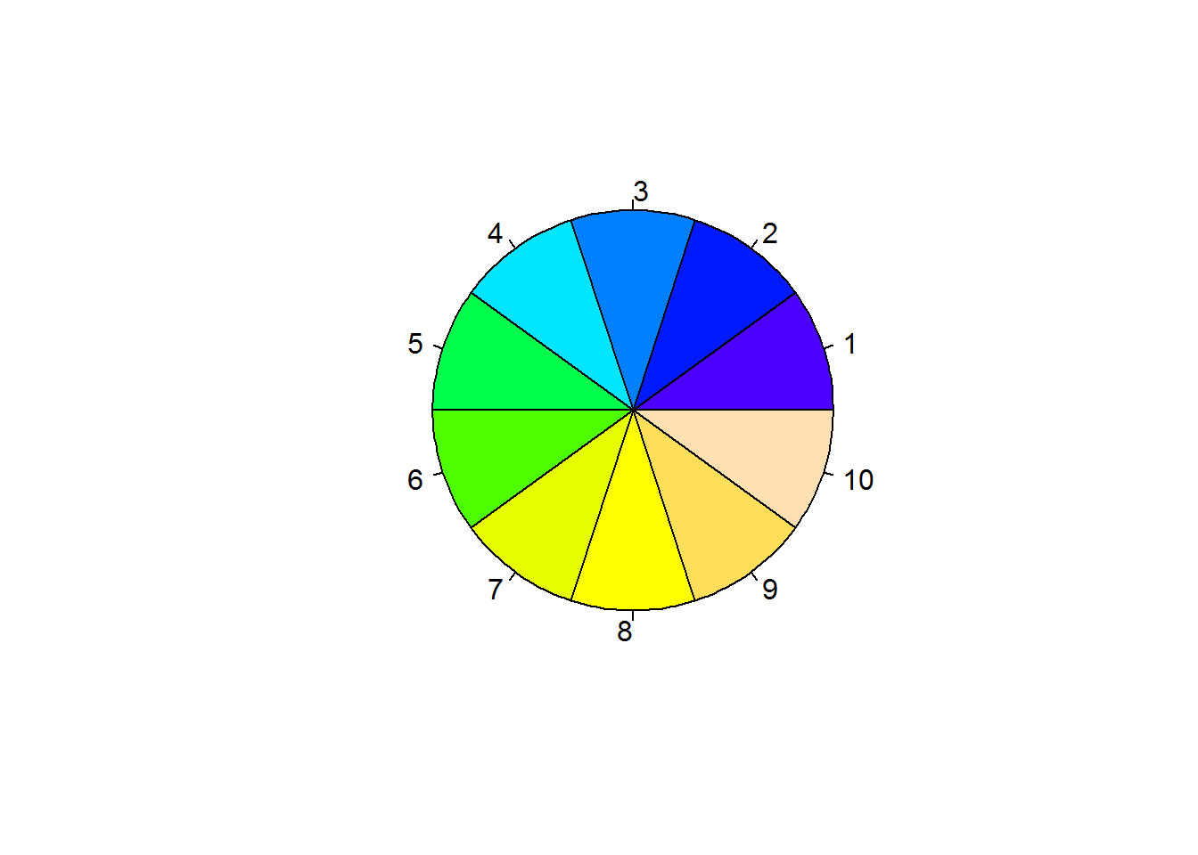
Change the N and see what kinds of colors you can get.
Text and symbols
Text and symbols are modified with cex. cex = symbol size relative to default (1),
cex.axis = magnification of axis
cex.lab, cex.main, cex.sub are all magnifications relative to cex setting.
font = 1, plain; 2 = bold; 3 = italic; 4 = bold italic; 5 = symbol.
font.lab, font.main. font.sub, etc. all change the font for that area. ps = text point/pixel size. Final text size is ps * cex
family = font family. E.g., serif, sans, mono, etc.
Examples:
plot(mtcars$wt.mt, mtcars$kpl,
     abline(lm(mtcars$kpl ~ mtcars$wt.mt)),
     main="Defaults")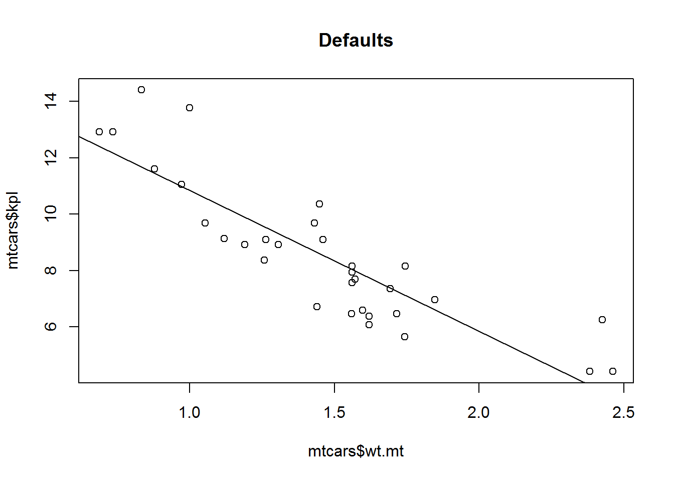
plot(mtcars$wt.mt, mtcars$kpl, cex = 2,
     abline(lm(mtcars$kpl ~ mtcars$wt.mt)),
     main="Big Symbols")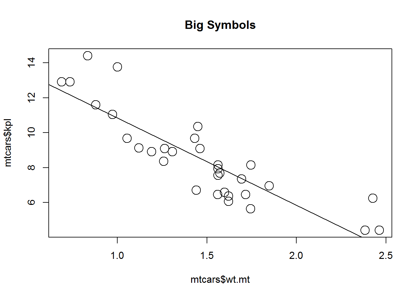
plot(mtcars$wt.mt, mtcars$kpl, cex = 1, font = 3,
     cex.main = .75, cex.lab = 2, abline(lm(mtcars$kpl ~ mtcars$wt.mt)),
     main="Italic Axes Labels, Large Text Legends, and Small Title")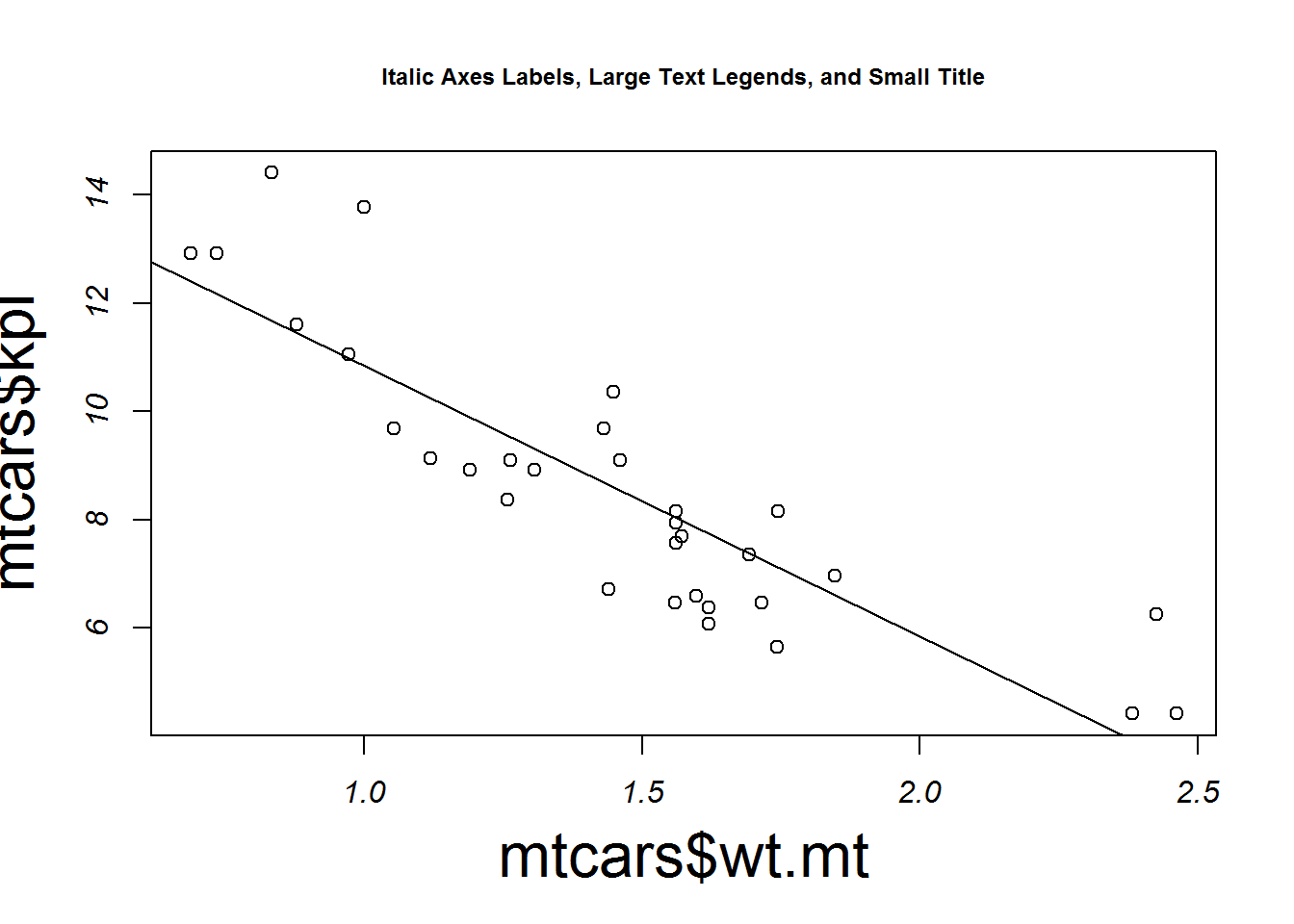
Dimensions
pin(width, height) changes the absolute size of the graph in inches. This makes the whole graph fit into a specific size and all other options are static. In other words, making the graph very big doesn’t necessarily make the text fit well. mai (bottom, left, top, right) are margins. You can change specific parts of how the graph is plotted with margins. They can get quite complex but there is a very nice guide available through http://research.stowers-institute.org/efg/R/Graphics/Basics/mar-oma/
Let’s put all this to use.
the par commands apply to both graphs but the inline only to that graph. We start by setting the dimensions of the graph to 5 inches wide by 4 inches tall. Then we make a thicker line and larger text with lch and cex. Finally, we make the axis text smaller and italicised.
par(pin=c(5,4))
par(lwd=2, cex=1.5)
par(cex.axis=.75, font.axis=3)
For each plot independently we will change the color and shape of the symbols
plot(mtcars$wt.mt, mtcars$kpl,
  abline(lm(mtcars$kpl ~ mtcars$wt.mt)),
  main="Defaults",
  pch = 19,
  col = "dodgerblue")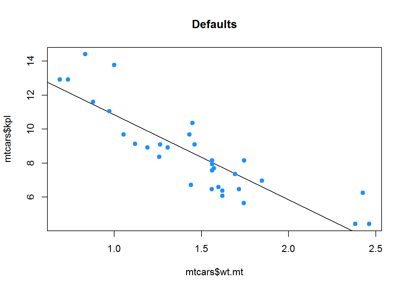
plot(mtcars$wt.mt, mtcars$kpl,
     abline(lm(mtcars$kpl ~ mtcars$wt.mt)),
     main="Defaults",
     pch = 23,
     col = "indianred")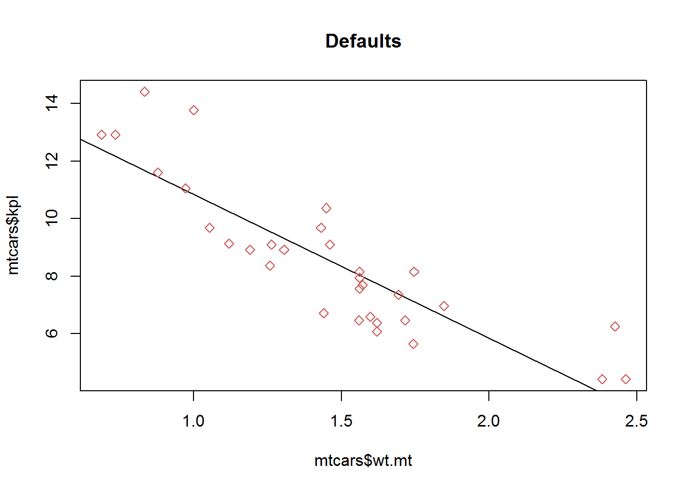
plot(mtcars$kpl, mtcars$hp, pch = 23, col="blue",
     abline(lm(mtcars$kpl ~ mtcars$hp)))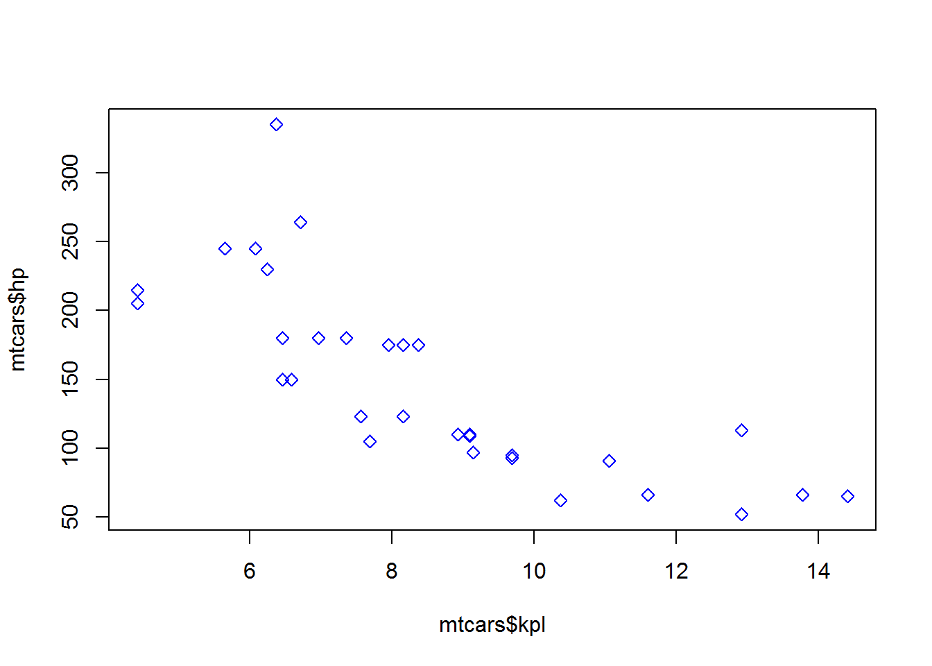
And reset the global parameters to their defaults.
par(defaultpar)Text customization
You can add text with main (title), sub (subtitle), xlab (x axis label), and ylab (y axis label).
plot(mtcars$kpl, mtcars$wt.mt,
     xlab = "Kilometers per Liter",
     ylab = "Weight in Metric Tons",
     main = "Scatterplot of K/L and WT",
     sub = "Data from mtcars")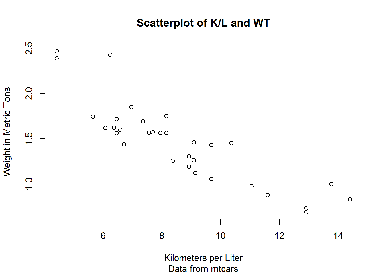
You can also annotate a graph with text and mtext. First we create a graph
Then, over the top of that graph we write at the intersections of wt.mt and kpl the name of the car. Since the name of the car is the name of the rows we can use row.names(mtcars). pos refers to the position that the text writes in we can use 4 to indicate to the right.
plot(mtcars$wt.mt, mtcars$kpl,
     main = "K/L vs. Weight",
     xlab = "Weight",
     ylab = "Kilometers per Liter",
     pch = 18,
     col = "steelblue")

text(mtcars$wt.mt, mtcars$kpl, row.names(mtcars), cex = .6, pos = 4, col = "Blue")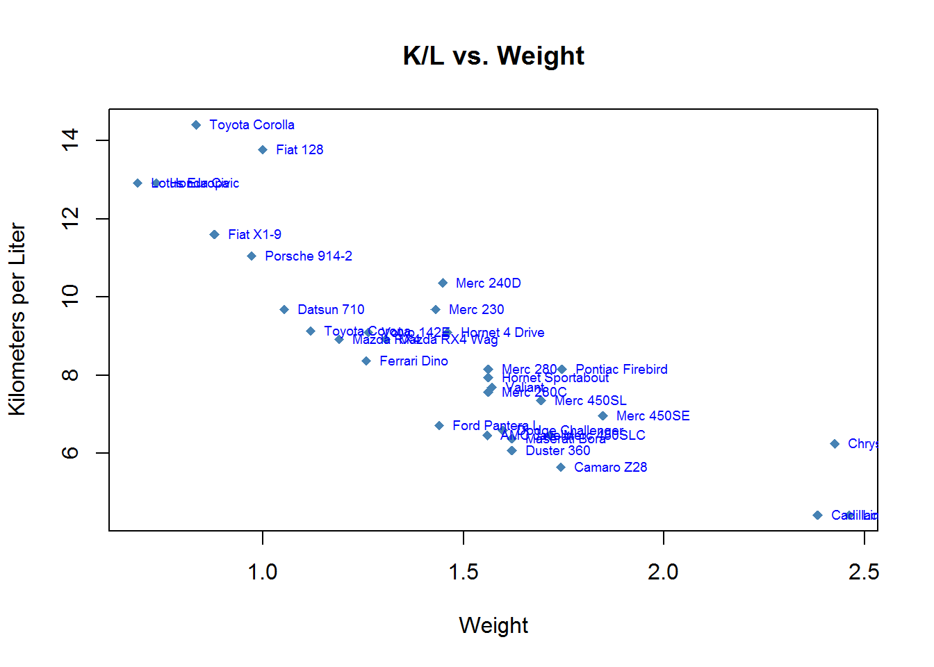
If we wanted to instead see how many cylenders each car has we would graph that just as easily by specifying that as the text to place in those positions.
plot(mtcars$wt.mt, mtcars$kpl,
     main = "K/L vs. Weight",
     xlab = "Weight",
     ylab = "Kilometers per Liter",
     pch = 18,
     col = "steelblue")

text(mtcars$wt.mt, mtcars$kpl, mtcars$cyl, cex = .6, pos = 4, col = "steelblue")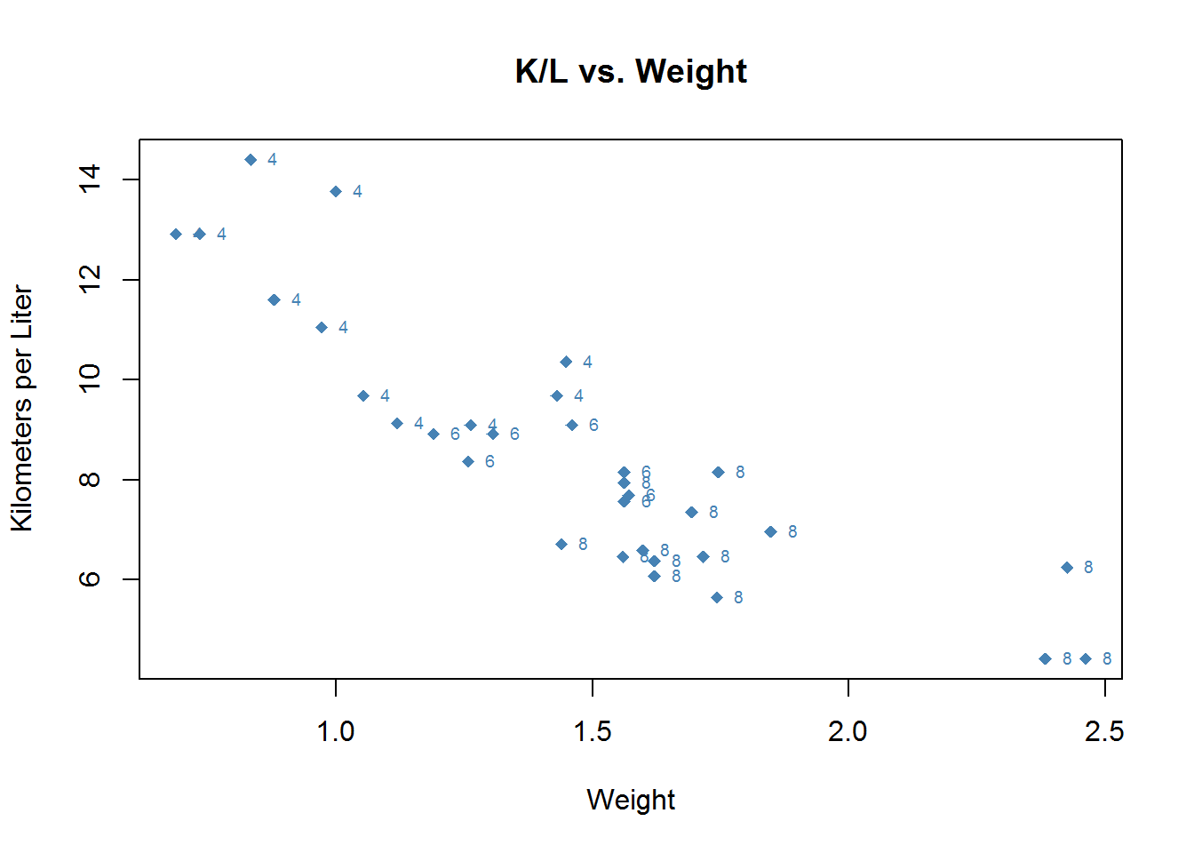
You can adjust the limits of the axies with xlim and ylim.
To set limits you give a list of lower coordinate and higher coordinate e.g., c(-5,32)
plot(mtcars$wt.mt, mtcars$kpl,
     main = "K/L vs. Weight",
     xlab = "Weight",
     ylab = "Kilometers per Liter",
     pch = 18,
     col = "Purple",
     xlim=c(0,10),
ylim=c(0,40)) 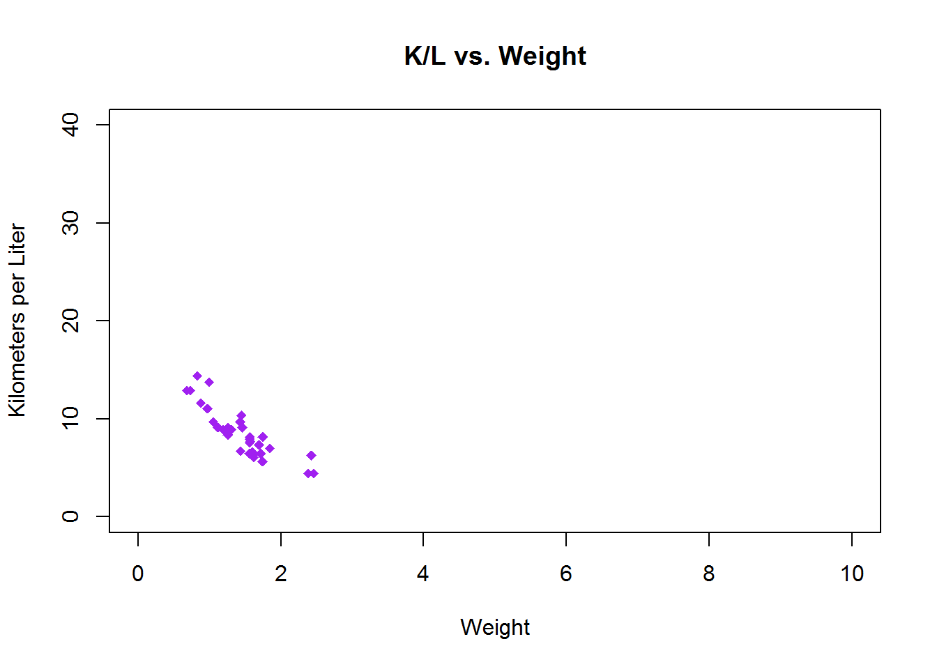
Combining Graphs
R can produce your plots in a matrix with par. One command in par is mfrow which stands for matrix plot where graphs are entered by row until filled. mfcol is the column version This wil automatically adjust things like cex of all options to be smaller in order to fit the graphs into the new matrix structure. Alternatively, you can use layout or split.screen. All the options have their strengths and weaknesses and none of them can be used together. Spend some time looking over the help documents for the three methods and choose the one that makes the most sense to you. I prefer layout which has the form:
layout(matrix, widths = rep.int(1, ncol(mat)), heights = rep.int(1, nrow(mat)), respect = FALSE). This creates a plot where the location of the next N figures are plotted. layout lets you choose exactly where on the plot things are appearing and how much room they take up. In the matrix you use an Integer to specify which plot goes where. For instance 1 is the next plot, 2 is the plot after that, etc. up until the number of plots you intend on being in the matrix a 0 means don’t use that area and a number in multiple places means use those cells for the same plot (span across the cells).
Let’s start with a matrix of plots where the next 4 plots get entered into their own cells. Lets have it so they are entered by row in a 2 by 2 fashion.
We can test if this is the layout we want with layout.show(n) where n is the number of plots we want to see (4 in this case.)
layout(matrix(c(1, 2, 3, 4), 2, 2, byrow = TRUE), respect = TRUE)

layout.show(4)
Okay, we have the arrangement we are looking for. Now we just create 4 plots and they will be filled in as they are plotted.
layout(matrix(c(1, 2, 3, 4), 2, 2, byrow = TRUE), respect = TRUE)
plot(mtcars$wt.mt, mtcars$kpl, main = "Scatterplot of K/L and WT")
plot(mtcars$wt.mt, mtcars$disp.c, main = "Scatterplot of Weight and Displacement")
hist(mtcars$wt.mt, main = "Histogram of Weight")
boxplot(mtcars$wt.mt, main = "Boxplot of Weight")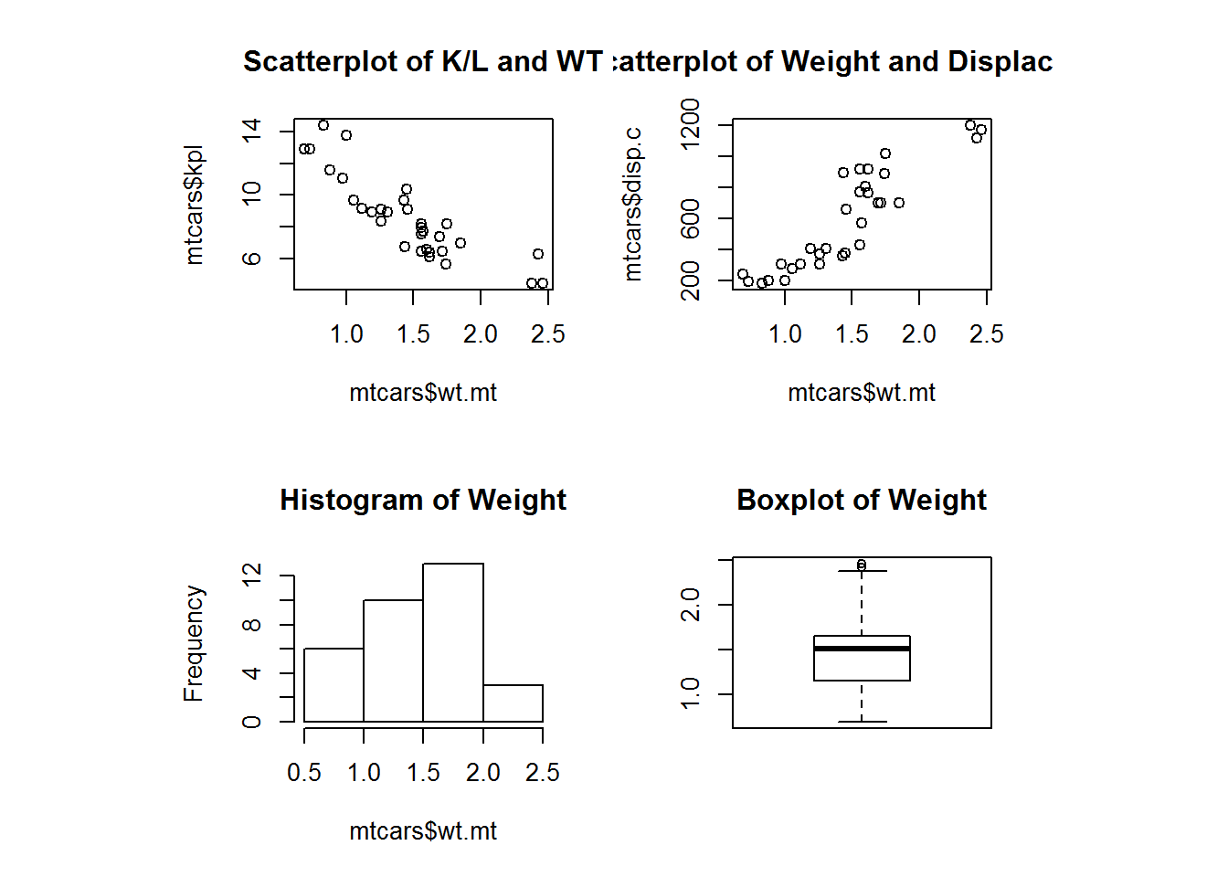
Then we need to reset back to the basics.
par(defaultpar)We could replicate most of what we have above but also assign the entire top row to 1 graph.
layout(matrix(c(1,1,2,3), 2, 2, byrow=TRUE))

layout.show(3)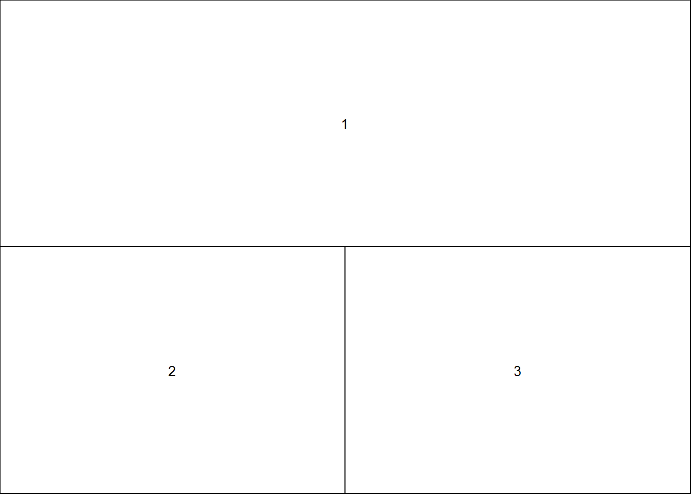
hist(mtcars$wt.mt, main = "Histogram of Weight")
hist(mtcars$kpl, main = "Histogram of Kilometers per Liter")
hist(mtcars$disp.c, main = "Histogram of Displacement")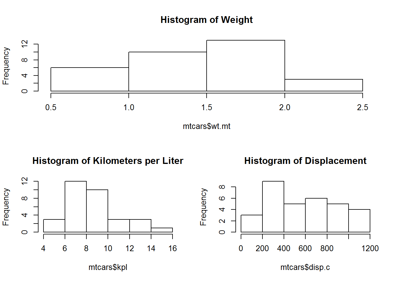
Then we need to reset back to the basics.
par(defaultpar)Finally, sometimes you will need a very fine control over the graphs. To do that we use fig to specify the exact coordinates for a plot to take up. fig is specified as a numerical vector of the form c(x1, x2, y1, y2) which gives the coordinates of the figure region in the display region of the device. If you set this you start a new plot, so to add to an existing plot use new = TRUE. The plotting area goes from 0 to 1 (think of it like percentages of the plotting area you want a figure to be inside). You can do negative and over 1 if you want to plot outside the typical range.
Let’s start with a plot that goes from 00% to 80% of X and 00% to 80% of Y. Then we will graph onto the 20% of the area above and to the right of those areas. What we want to create are density plots around a scatter plot with a regression line.
After that we specify a graph to fill the rest of the space. This is where it can begin to get tricky. Since the graph we want will span the same x that is easy (00 and 0.8). But, the graph on the y axis will be small if we tell it to take only the remaining space. So, it’s best to play around with the exact dimensions for output that you think looks good. If you are using RStudio don’t rely on the preview since it will scale to the dimensions of your monitor. You will need to use zoom or save the graph in order to get the best dimensions for display or print.
par(fig=c(0, 0.8, 0, 0.8)) #Specify coordinates for plot

layout.show(1) #Check if this is the right plotting area.
plot(mtcars$wt.mt, mtcars$kpl,
     xlab = "Weight in Metric Tons",
     ylab = "Kilometers per Liter",
     col = "steelblue", pch = 10) #Create our plot.

par(fig=c(0, 0.8, 0.55, 1), new = TRUE)

# For the boxplot we can flip the graph with horizontal = TRUE and
# disable the display of the axes with axes = FALSE.

boxplot(mtcars$wt.mt, horizontal = TRUE, axes = FALSE, col = "steelblue2")

par(fig=c(0.7, 0.95, 0, 0.8), new = TRUE)
boxplot(mtcars$kpl, axes=FALSE, col = "steelblue2")

mtext("Scatterplot of K/L and Weight with Density Boxplots", side = 3, outer = TRUE,
      col = "mediumvioletred", line = -3, cex = 1.5)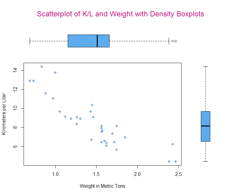
Finally, we can add a title with mtext (if we used main in the original graph it would overlay the position we want the boxplot to be in). We use side to say where it should be positioned in this case 3 which is the top. Then we can tell it that graphing outside the plot area is fine with outer = TRUE. Last, we need to offset the title a bit with line = -3. This too will be a little trial and error in order to find a good position for you, based on the size of the graph you are constructing.
par(defaultpar)I, frankly, do not like using fig. I find the plots never quite turn out how you want and there is simply too much fiddling around and inexactness. Usually, if you want a complex plot it can be accomplished easier through the use of packages. Those packages usually come with a better way to print and save the plot as well.
Now that you have become an expert on creating graphs with Base-R why not give the lab a try? It’s a rather simple exercise where you try and replicate a few graphs by using what you learned above.
Lab 2: https://docs.google.com/document/d/1g3nQ1a0shnvXC-PkPcAYKV5fuDWMxMORVQG5armCbXw/edit?usp=sharing
Answers: https://drive.google.com/file/d/0BzzRhb-koTrLNnpOZXhNMEplVjA/view?usp=sharing
If you are having issues with the answers try downloading them and opening them in your browser of choice.