I just finished up teaching a semester long course on R programming in the social sciences. After gathering a lot of feedback from the students and the notes I took I am going back through the course and making modifications and extensions on some topics. As I modify the course and shape it to be even better I will be posting syntax and output for people to follow along and labs for testing abilities!
The following series of Teaching and Learning R is aimed at helping someone start from knowing very little about R and computer programming in general who has a basic statistical knowledge (General Linear Model) understand how to properly format data, graph, do statistical analyses, and output from R into a usable format. This includes publication quality graphs and tables. If you have any comments or feedback please don’t hesitate to email me directly or leave a comment on the blog!
Please try to write out the syntax yourself. Try and play around a little and see what you get and what the boundaries are. At the end of the lesson is a lab to help test your skills!
Lesson 1: Data Structures and R Syntax
Scott Withrow
June 23, 2015
Syntax for R is similar to a computer programming language. You may use whatever rules you want within certain limits. R is whitespace insensitive so you can use as many or as few spaces as you wish. R is case sensitive so you will need to be sure you are capitalizing things consistently. Although you may do whatever you wish with your syntax there are a number of rules that will make your code easier to read, follow, and understand. Particularly, I believe that having spaces around operators, spaces after all commas, and a consistent methodology for naming variables to be the most essential things to get used to. I would suggest Hadley Wickham’s R style guide (http://adv-r.had.co.nz/Style.html). Read through that document and commit it to memory and you will have an easier time with R programming. Google also maintains a useful style guide (http://google-styleguide.googlecode.com/svn/trunk/Rguide.xml).
Use comments for everything! You don’t know when you will want to review code or give code to someone else. A good description of what you were thinking when you wrote it and what you hoped to acomplish and why you did what you did will save you a lot of time in the long run. Writing comments in R-Studio is easy. Just type a # and follow it with a long line of text. Then highlight the line of text and click reflow comment in the code menu. In Windows the shortcut is ctrl+shift+/.
R is composed of a number of components. You have the Console where everything is run. In a text or Base-R you would do most of your code here. This is a great place to do simple analyses, quick plots, or to test things out. You can hit the up arrow while in the console to see past entries. This is the lower left window in RStudio. You have a syntax view available where you can spend more time structuring syntax and flows. This is generally where you will do most of your work and is the upper left window in RStudio. When a variable is created, a dataset loaded, or something is saved it is stored in the workspace. Think of this like a desktop where all your documents are located. This is represented as “Environemnt” in the upper right corner in RStudio (it’s basically a constant display of str()). Last there are a number of objects that will be created in any analysis (e.g., plots) which will be popups in Base-R and are stored in the lower right window in RStudio.
There is a large amount of information and guides available for running R through the R Project Manuals page (http://cran.r-project.org/). I would recomend reading and following along with them. Particularly the beginning of “An Introduction to R” and “Data Import / Export” as those are very helpful topics. You can find a lot of help through a number of websites as well. The most popular place to ask R questions is at stackoverflow (http://stackoverflow.com/questions/tagged/r). There is a smaller but still helpful community you can access through reddit as well (http://www.reddit.com/r/rstats). For either of these websites you can ask basic and complex questions but you should try searching the websites for similar questions first, people can get quite grumpy with repeated questions that have already been answered. If you have a new question try and provide example data either as a download or give syntax that creates a small dataset like what you are working with and what you expect the output to look like when you are done. If you don’t the first responses to your question will be someone telling you to do that. Finally, you can access help manuals for each function with help(command) or ?command. You can even do a web search with ??command. Try it out ?sum
Vectors
x <- c(10.4, 5.6, 3.1, 6.4, 21.7) #c stands for concatenated listOR
assign("x", c(10.4, 5.6, 3.1, 6.4, 21.7))<- is therefore a shortcut for assign. -> and = also assign as long as the arrow points the correct direction. Usually the = are not used as much as the arrows since you should always be sure which direction you are doing your assignments.
If we do arithmetic on this vector it doesn’t change the vector
1 / x## [1] 0.09615385 0.17857143 0.32258065 0.15625000 0.04608295x + 10## [1] 20.4 15.6 13.1 16.4 31.7x * 100## [1] 1040 560 310 640 2170Only if we assign it a variable name is it stored.
We can also use vectors within vectors
y <- c(x, 0, x)
y
## [1] 10.4 5.6 3.1 6.4 21.7 0.0 10.4 5.6 3.1 6.4 21.7R will always make vector arithmetic the length of the longest vector
v <- 2 * x + y + 1## Warning in 2 * x + y: longer object length is not a multiple of shorter
## object lengthv## [1] 32.2 17.8 10.3 20.2 66.1 21.8 22.6 12.8 16.9 50.8 43.5x is repeated 2.2 times, y once and 1 11 times
You can also do arithmetic between parts of vectors
x[2] * x[4]## [1] 35.84you can also have vectors of characters
a <- c("one", "two", "three")
a
## [1] "one" "two" "three"and logical
b <- c(TRUE, TRUE, TRUE, FALSE, TRUE, FALSE)
b
## [1] TRUE TRUE TRUE FALSE TRUE FALSEVector Referencing
vector[position]
x[2] #second position## [1] 5.6x[c(2, 5)] #second and fifth position## [1] 5.6 21.7R also supports a through statement
x[2:6] #positions 2 through 6 (returns an NA because 6 doesn't exist)## [1] 5.6 3.1 6.4 21.7 NAMatrices
matrix(data = NA, nrow = numberofrows, ncol = numberofcolumns, byrow = FALSE, dimnames = c(rownames, colnames))
c <- matrix(1:20, nrow = 5, ncol = 4) add byrow = TRUE to fill in the matrix by rows
c## [,1] [,2] [,3] [,4]
## [1,] 1 6 11 16
## [2,] 2 7 12 17
## [3,] 3 8 13 18
## [4,] 4 9 14 19
## [5,] 5 10 15 20Matrix referencing
matrix[row position, col position]
A blank means all
c[1, ] #all of row 1## [1] 1 6 11 16c[, 1] #all of column 1## [1] 1 2 3 4 5c[5, 2] #cell from row 5 column 2## [1] 10c[c(2, 5), 4] #rows 2 and 5 in column 4## [1] 17 20c[1:3, 2:3] #rows 1 through 3 and columns 2 through 3## [,1] [,2]
## [1,] 6 11
## [2,] 7 12
## [3,] 8 13Arrays
array(data = NA, dim = length(data), dimnames = NULL)
dim1 <- c("A1", "A2")
dim2 <- c("B1", "B2", "B3")
dim3 <- c("C1", "C2", "C3", "C4")

z <- array(1:24, c(2, 3, 4), dimnames=list(dim1, dim2, dim3))
z
## , , C1
##
## B1 B2 B3
## A1 1 3 5
## A2 2 4 6
##
## , , C2
##
## B1 B2 B3
## A1 7 9 11
## A2 8 10 12
##
## , , C3
##
## B1 B2 B3
## A1 13 15 17
## A2 14 16 18
##
## , , C4
##
## B1 B2 B3
## A1 19 21 23
## A2 20 22 24Array referencing
array[row position, col position, dimension position]
z[1, 2, 1:3]## C1 C2 C3
## 3 9 15Data Frames
Similar to what you would expect to work with in SPSS, SAS, Excel, etc.
Sepallength <- c(5.1, 4.9, 7, 6.4, 6.3, 5.8)
Sepalwidth <- c(3.5, 3.0, 3.2, 3.2, 3.3, 2.7)
Petallength <- c(1.4, 1.4, 4.7, 4.5, 6.0, 5.1)
Petalwidth <- c(.2, .2,1.4, 1.5,  2.5, 1.9)
Species <- c("I. setosa", "I. setosa", "I. versicolor", "I. versicolor", "I. virginica", "I. virginica")
Firis <- data.frame(Sepallength, Sepalwidth, Petallength, Petalwidth, Species)
Firis
## Sepallength Sepalwidth Petallength Petalwidth Species
## 1 5.1 3.5 1.4 0.2 I. setosa
## 2 4.9 3.0 1.4 0.2 I. setosa
## 3 7.0 3.2 4.7 1.4 I. versicolor
## 4 6.4 3.2 4.5 1.5 I. versicolor
## 5 6.3 3.3 6.0 2.5 I. virginica
## 6 5.8 2.7 5.1 1.9 I. virginicaData frame referencing
dataframe[row position, col position]
Unlike with matrices you can also use column names
Firis[c(1, 3)] #Comparing Sepal Length and Petal Length## Sepallength Petallength
## 1 5.1 1.4
## 2 4.9 1.4
## 3 7.0 4.7
## 4 6.4 4.5
## 5 6.3 6.0
## 6 5.8 5.1Instead of counting columns we can refer to column name
Firis[c("Sepallength", "Petallength")] ## Sepallength Petallength
## 1 5.1 1.4
## 2 4.9 1.4
## 3 7.0 4.7
## 4 6.4 4.5
## 5 6.3 6.0
## 6 5.8 5.1The most common way we will reference something is with a $. A $ means within. We can call a single variable with dataframe$variable_name
Firis$Sepalwidth ## [1] 3.5 3.0 3.2 3.2 3.3 2.7selecting a single variable is very important, especially when we want to cross tabulate
table(Firis$Sepalwidth, Firis$Species)##
## I. setosa I. versicolor I. virginica
## 2.7 0 0 1
## 3 1 0 0
## 3.2 0 2 0
## 3.3 0 0 1
## 3.5 1 0 0I have a little secret. The iris data in it’s entirety already exists inside Base R. Lets clear the workspace then load up that data.
rm(list=ls())There is a lot of data so we can get partial pictures of the dataset with
head(iris) #first 6 rows## Sepal.Length Sepal.Width Petal.Length Petal.Width Species
## 1 5.1 3.5 1.4 0.2 setosa
## 2 4.9 3.0 1.4 0.2 setosa
## 3 4.7 3.2 1.3 0.2 setosa
## 4 4.6 3.1 1.5 0.2 setosa
## 5 5.0 3.6 1.4 0.2 setosa
## 6 5.4 3.9 1.7 0.4 setosatail(iris) #last 6 rows## Sepal.Length Sepal.Width Petal.Length Petal.Width Species
## 145 6.7 3.3 5.7 2.5 virginica
## 146 6.7 3.0 5.2 2.3 virginica
## 147 6.3 2.5 5.0 1.9 virginica
## 148 6.5 3.0 5.2 2.0 virginica
## 149 6.2 3.4 5.4 2.3 virginica
## 150 5.9 3.0 5.1 1.8 virginicasummary(iris) #summary statistics for each column## Sepal.Length Sepal.Width Petal.Length Petal.Width
## Min. :4.300 Min. :2.000 Min. :1.000 Min. :0.100
## 1st Qu.:5.100 1st Qu.:2.800 1st Qu.:1.600 1st Qu.:0.300
## Median :5.800 Median :3.000 Median :4.350 Median :1.300
## Mean :5.843 Mean :3.057 Mean :3.758 Mean :1.199
## 3rd Qu.:6.400 3rd Qu.:3.300 3rd Qu.:5.100 3rd Qu.:1.800
## Max. :7.900 Max. :4.400 Max. :6.900 Max. :2.500
## Species
## setosa :50
## versicolor:50
## virginica :50
##
##
## str(iris) #the types of variables in the data frame## 'data.frame': 150 obs. of 5 variables:
## $ Sepal.Length: num 5.1 4.9 4.7 4.6 5 5.4 4.6 5 4.4 4.9 ...
## $ Sepal.Width : num 3.5 3 3.2 3.1 3.6 3.9 3.4 3.4 2.9 3.1 ...
## $ Petal.Length: num 1.4 1.4 1.3 1.5 1.4 1.7 1.4 1.5 1.4 1.5 ...
## $ Petal.Width : num 0.2 0.2 0.2 0.2 0.2 0.4 0.3 0.2 0.2 0.1 ...
## $ Species : Factor w/ 3 levels "setosa","versicolor",..: 1 1 1 1 1 1 1 1 1 1 ...We could use table(iris$Sepal.Width, iris$Species) to see an expanded version of the above table or we can make sure R will use the iris data. We can do that with attach(dataframe). This loads all the variables in the dataset into the global environment so they are accessable by all functions without telling them what dataset they belong to. However, variables that you create and add to the dataset will NOT be automatically attached. Most programmers, myself included, would recommend not using attach.
attach(iris)
table(Sepal.Width, Species)
## Species
## Sepal.Width setosa versicolor virginica
## 2 0 1 0
## 2.2 0 2 1
## 2.3 1 3 0
## 2.4 0 3 0
## 2.5 0 4 4
## 2.6 0 3 2
## 2.7 0 5 4
## 2.8 0 6 8
## 2.9 1 7 2
## 3 6 8 12
## 3.1 4 3 4
## 3.2 5 3 5
## 3.3 2 1 3
## 3.4 9 1 2
## 3.5 6 0 0
## 3.6 3 0 1
## 3.7 3 0 0
## 3.8 4 0 2
## 3.9 2 0 0
## 4 1 0 0
## 4.1 1 0 0
## 4.2 1 0 0
## 4.4 1 0 0you can reverse attach with detach()
detach(iris)You can also temporarily do a series of operations in a data frame
with(iris, {
  plot(Species, Petal.Length, main="Petal Length by Species")
})
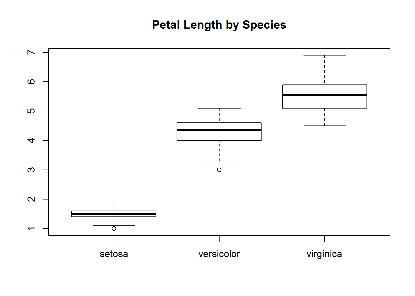
The limitation of with is that it only considers the variables you specify and doesn’t call the dataframe. We can call the dataframe with within.
within(iris, {
  Petal.Area <- Petal.Length * Petal.Width #Create the variable
})
## Sepal.Length Sepal.Width Petal.Length Petal.Width Species
## 1 5.1 3.5 1.4 0.2 setosa
## 2 4.9 3.0 1.4 0.2 setosa
## 3 4.7 3.2 1.3 0.2 setosa
## 4 4.6 3.1 1.5 0.2 setosa
## 5 5.0 3.6 1.4 0.2 setosa
## 6 5.4 3.9 1.7 0.4 setosa
## 7 4.6 3.4 1.4 0.3 setosa
## 8 5.0 3.4 1.5 0.2 setosa
## 9 4.4 2.9 1.4 0.2 setosa
## 10 4.9 3.1 1.5 0.1 setosa
## 11 5.4 3.7 1.5 0.2 setosa
## 12 4.8 3.4 1.6 0.2 setosa
## 13 4.8 3.0 1.4 0.1 setosa
## 14 4.3 3.0 1.1 0.1 setosa
## 15 5.8 4.0 1.2 0.2 setosa
## 16 5.7 4.4 1.5 0.4 setosa
## 17 5.4 3.9 1.3 0.4 setosa
## 18 5.1 3.5 1.4 0.3 setosa
## 19 5.7 3.8 1.7 0.3 setosa
## 20 5.1 3.8 1.5 0.3 setosa
## 21 5.4 3.4 1.7 0.2 setosa
## 22 5.1 3.7 1.5 0.4 setosa
## 23 4.6 3.6 1.0 0.2 setosa
## 24 5.1 3.3 1.7 0.5 setosa
## 25 4.8 3.4 1.9 0.2 setosa
## 26 5.0 3.0 1.6 0.2 setosa
## 27 5.0 3.4 1.6 0.4 setosa
## 28 5.2 3.5 1.5 0.2 setosa
## 29 5.2 3.4 1.4 0.2 setosa
## 30 4.7 3.2 1.6 0.2 setosa
## 31 4.8 3.1 1.6 0.2 setosa
## 32 5.4 3.4 1.5 0.4 setosa
## 33 5.2 4.1 1.5 0.1 setosa
## 34 5.5 4.2 1.4 0.2 setosa
## 35 4.9 3.1 1.5 0.2 setosa
## 36 5.0 3.2 1.2 0.2 setosa
## 37 5.5 3.5 1.3 0.2 setosa
## 38 4.9 3.6 1.4 0.1 setosa
## 39 4.4 3.0 1.3 0.2 setosa
## 40 5.1 3.4 1.5 0.2 setosa
## 41 5.0 3.5 1.3 0.3 setosa
## 42 4.5 2.3 1.3 0.3 setosa
## 43 4.4 3.2 1.3 0.2 setosa
## 44 5.0 3.5 1.6 0.6 setosa
## 45 5.1 3.8 1.9 0.4 setosa
## 46 4.8 3.0 1.4 0.3 setosa
## 47 5.1 3.8 1.6 0.2 setosa
## 48 4.6 3.2 1.4 0.2 setosa
## 49 5.3 3.7 1.5 0.2 setosa
## 50 5.0 3.3 1.4 0.2 setosa
## 51 7.0 3.2 4.7 1.4 versicolor
## 52 6.4 3.2 4.5 1.5 versicolor
## 53 6.9 3.1 4.9 1.5 versicolor
## 54 5.5 2.3 4.0 1.3 versicolor
## 55 6.5 2.8 4.6 1.5 versicolor
## 56 5.7 2.8 4.5 1.3 versicolor
## 57 6.3 3.3 4.7 1.6 versicolor
## 58 4.9 2.4 3.3 1.0 versicolor
## 59 6.6 2.9 4.6 1.3 versicolor
## 60 5.2 2.7 3.9 1.4 versicolor
## 61 5.0 2.0 3.5 1.0 versicolor
## 62 5.9 3.0 4.2 1.5 versicolor
## 63 6.0 2.2 4.0 1.0 versicolor
## 64 6.1 2.9 4.7 1.4 versicolor
## 65 5.6 2.9 3.6 1.3 versicolor
## 66 6.7 3.1 4.4 1.4 versicolor
## 67 5.6 3.0 4.5 1.5 versicolor
## 68 5.8 2.7 4.1 1.0 versicolor
## 69 6.2 2.2 4.5 1.5 versicolor
## 70 5.6 2.5 3.9 1.1 versicolor
## 71 5.9 3.2 4.8 1.8 versicolor
## 72 6.1 2.8 4.0 1.3 versicolor
## 73 6.3 2.5 4.9 1.5 versicolor
## 74 6.1 2.8 4.7 1.2 versicolor
## 75 6.4 2.9 4.3 1.3 versicolor
## 76 6.6 3.0 4.4 1.4 versicolor
## 77 6.8 2.8 4.8 1.4 versicolor
## 78 6.7 3.0 5.0 1.7 versicolor
## 79 6.0 2.9 4.5 1.5 versicolor
## 80 5.7 2.6 3.5 1.0 versicolor
## 81 5.5 2.4 3.8 1.1 versicolor
## 82 5.5 2.4 3.7 1.0 versicolor
## 83 5.8 2.7 3.9 1.2 versicolor
## 84 6.0 2.7 5.1 1.6 versicolor
## 85 5.4 3.0 4.5 1.5 versicolor
## 86 6.0 3.4 4.5 1.6 versicolor
## 87 6.7 3.1 4.7 1.5 versicolor
## 88 6.3 2.3 4.4 1.3 versicolor
## 89 5.6 3.0 4.1 1.3 versicolor
## 90 5.5 2.5 4.0 1.3 versicolor
## 91 5.5 2.6 4.4 1.2 versicolor
## 92 6.1 3.0 4.6 1.4 versicolor
## 93 5.8 2.6 4.0 1.2 versicolor
## 94 5.0 2.3 3.3 1.0 versicolor
## 95 5.6 2.7 4.2 1.3 versicolor
## 96 5.7 3.0 4.2 1.2 versicolor
## 97 5.7 2.9 4.2 1.3 versicolor
## 98 6.2 2.9 4.3 1.3 versicolor
## 99 5.1 2.5 3.0 1.1 versicolor
## 100 5.7 2.8 4.1 1.3 versicolor
## 101 6.3 3.3 6.0 2.5 virginica
## 102 5.8 2.7 5.1 1.9 virginica
## 103 7.1 3.0 5.9 2.1 virginica
## 104 6.3 2.9 5.6 1.8 virginica
## 105 6.5 3.0 5.8 2.2 virginica
## 106 7.6 3.0 6.6 2.1 virginica
## 107 4.9 2.5 4.5 1.7 virginica
## 108 7.3 2.9 6.3 1.8 virginica
## 109 6.7 2.5 5.8 1.8 virginica
## 110 7.2 3.6 6.1 2.5 virginica
## 111 6.5 3.2 5.1 2.0 virginica
## 112 6.4 2.7 5.3 1.9 virginica
## 113 6.8 3.0 5.5 2.1 virginica
## 114 5.7 2.5 5.0 2.0 virginica
## 115 5.8 2.8 5.1 2.4 virginica
## 116 6.4 3.2 5.3 2.3 virginica
## 117 6.5 3.0 5.5 1.8 virginica
## 118 7.7 3.8 6.7 2.2 virginica
## 119 7.7 2.6 6.9 2.3 virginica
## 120 6.0 2.2 5.0 1.5 virginica
## 121 6.9 3.2 5.7 2.3 virginica
## 122 5.6 2.8 4.9 2.0 virginica
## 123 7.7 2.8 6.7 2.0 virginica
## 124 6.3 2.7 4.9 1.8 virginica
## 125 6.7 3.3 5.7 2.1 virginica
## 126 7.2 3.2 6.0 1.8 virginica
## 127 6.2 2.8 4.8 1.8 virginica
## 128 6.1 3.0 4.9 1.8 virginica
## 129 6.4 2.8 5.6 2.1 virginica
## 130 7.2 3.0 5.8 1.6 virginica
## 131 7.4 2.8 6.1 1.9 virginica
## 132 7.9 3.8 6.4 2.0 virginica
## 133 6.4 2.8 5.6 2.2 virginica
## 134 6.3 2.8 5.1 1.5 virginica
## 135 6.1 2.6 5.6 1.4 virginica
## 136 7.7 3.0 6.1 2.3 virginica
## 137 6.3 3.4 5.6 2.4 virginica
## 138 6.4 3.1 5.5 1.8 virginica
## 139 6.0 3.0 4.8 1.8 virginica
## 140 6.9 3.1 5.4 2.1 virginica
## 141 6.7 3.1 5.6 2.4 virginica
## 142 6.9 3.1 5.1 2.3 virginica
## 143 5.8 2.7 5.1 1.9 virginica
## 144 6.8 3.2 5.9 2.3 virginica
## 145 6.7 3.3 5.7 2.5 virginica
## 146 6.7 3.0 5.2 2.3 virginica
## 147 6.3 2.5 5.0 1.9 virginica
## 148 6.5 3.0 5.2 2.0 virginica
## 149 6.2 3.4 5.4 2.3 virginica
## 150 5.9 3.0 5.1 1.8 virginica
## Petal.Area
## 1 0.28
## 2 0.28
## 3 0.26
## 4 0.30
## 5 0.28
## 6 0.68
## 7 0.42
## 8 0.30
## 9 0.28
## 10 0.15
## 11 0.30
## 12 0.32
## 13 0.14
## 14 0.11
## 15 0.24
## 16 0.60
## 17 0.52
## 18 0.42
## 19 0.51
## 20 0.45
## 21 0.34
## 22 0.60
## 23 0.20
## 24 0.85
## 25 0.38
## 26 0.32
## 27 0.64
## 28 0.30
## 29 0.28
## 30 0.32
## 31 0.32
## 32 0.60
## 33 0.15
## 34 0.28
## 35 0.30
## 36 0.24
## 37 0.26
## 38 0.14
## 39 0.26
## 40 0.30
## 41 0.39
## 42 0.39
## 43 0.26
## 44 0.96
## 45 0.76
## 46 0.42
## 47 0.32
## 48 0.28
## 49 0.30
## 50 0.28
## 51 6.58
## 52 6.75
## 53 7.35
## 54 5.20
## 55 6.90
## 56 5.85
## 57 7.52
## 58 3.30
## 59 5.98
## 60 5.46
## 61 3.50
## 62 6.30
## 63 4.00
## 64 6.58
## 65 4.68
## 66 6.16
## 67 6.75
## 68 4.10
## 69 6.75
## 70 4.29
## 71 8.64
## 72 5.20
## 73 7.35
## 74 5.64
## 75 5.59
## 76 6.16
## 77 6.72
## 78 8.50
## 79 6.75
## 80 3.50
## 81 4.18
## 82 3.70
## 83 4.68
## 84 8.16
## 85 6.75
## 86 7.20
## 87 7.05
## 88 5.72
## 89 5.33
## 90 5.20
## 91 5.28
## 92 6.44
## 93 4.80
## 94 3.30
## 95 5.46
## 96 5.04
## 97 5.46
## 98 5.59
## 99 3.30
## 100 5.33
## 101 15.00
## 102 9.69
## 103 12.39
## 104 10.08
## 105 12.76
## 106 13.86
## 107 7.65
## 108 11.34
## 109 10.44
## 110 15.25
## 111 10.20
## 112 10.07
## 113 11.55
## 114 10.00
## 115 12.24
## 116 12.19
## 117 9.90
## 118 14.74
## 119 15.87
## 120 7.50
## 121 13.11
## 122 9.80
## 123 13.40
## 124 8.82
## 125 11.97
## 126 10.80
## 127 8.64
## 128 8.82
## 129 11.76
## 130 9.28
## 131 11.59
## 132 12.80
## 133 12.32
## 134 7.65
## 135 7.84
## 136 14.03
## 137 13.44
## 138 9.90
## 139 8.64
## 140 11.34
## 141 13.44
## 142 11.73
## 143 9.69
## 144 13.57
## 145 14.25
## 146 11.96
## 147 9.50
## 148 10.40
## 149 12.42
## 150 9.18Notice how it prints out all the data with our new column?
Compare that to with.
with(iris, {
  Petal.Area <- Petal.Length * Petal.Width
})
Nothing is printed.
In order to save this data we need to assign it back to the dataframe or to a new dataframe.
within(iris, {
  Petal.Area <- Petal.Length * Petal.Width
}) -> iris #Assign the variable to iris dataframe
head(iris)
## Sepal.Length Sepal.Width Petal.Length Petal.Width Species Petal.Area
## 1 5.1 3.5 1.4 0.2 setosa 0.28
## 2 4.9 3.0 1.4 0.2 setosa 0.28
## 3 4.7 3.2 1.3 0.2 setosa 0.26
## 4 4.6 3.1 1.5 0.2 setosa 0.30
## 5 5.0 3.6 1.4 0.2 setosa 0.28
## 6 5.4 3.9 1.7 0.4 setosa 0.68We now have Petal.Area as a column in our dataframe.
If we used with we would only have our new variable
with(iris, {
  Petal.Area <- Petal.Length * Petal.Width
}) -> iris2
head(iris2)
## [1] 0.28 0.28 0.26 0.30 0.28 0.68Factors
R will automatically create dummy codes for text entries if you turn them into factors. Factors can be complex at first but they are quite powerful. You can read more about how R deals with factors at http://www.stat.berkeley.edu/~s133/factors.html
diabetes <- c("Type1", "Type2", "Type1", "Type2")
diabetes
## [1] "Type1" "Type2" "Type1" "Type2"class(diabetes) #class tells us what type of variable we have## [1] "character"str(diabetes)## chr [1:4] "Type1" "Type2" "Type1" "Type2"diabetes <- factor(diabetes)
diabetes #notice how the "" are gone## [1] Type1 Type2 Type1 Type2
## Levels: Type1 Type2class(diabetes)## [1] "factor"str(diabetes) ## Factor w/ 2 levels "Type1","Type2": 1 2 1 2You can see the codes now. Codes are applied as the catagories in alphabetical order. This is a NOMINAL variable.
rating <- c("Strongly Disagree", "Disagree", "Agree", "Strongly Agree")
rating <- factor(rating)
rating
## [1] Strongly Disagree Disagree Agree Strongly Agree
## Levels: Agree Disagree Strongly Agree Strongly Disagreeclass(rating)## [1] "factor"str(rating) #notice agree is 1, then disagree is 2, etc.## Factor w/ 4 levels "Agree","Disagree",..: 4 2 1 3To make this an ORDINAL variable we need to use ordered = TRUE and levels
rating <- factor(c("Strongly Disagree", "Disagree", "Agree", "Strongly Agree"),
                 ordered=TRUE,
                 levels=c("Strongly Disagree", "Disagree", "Agree", "Strongly Agree"))
rating
## [1] Strongly Disagree Disagree Agree Strongly Agree
## Levels: Strongly Disagree < Disagree < Agree < Strongly Agreeclass(rating)## [1] "ordered" "factor"str(rating)## Ord.factor w/ 4 levels "Strongly Disagree"<..: 1 2 3 4If you have numeric data and you want to make it a categorical variable rating <- factor(rating, levels=(c(1:4)), labels=c(“Strongly Disagree”, “Disagree”, “Agree”, “Strongly Agree”))
Let’s pretend like someone rated how much they liked those irises. We can use a randomizer to assign these values for us quickly. If we want it to be a reporoducable randomization we can use set.seed which tells R the next time you randomize something use this randomizer signature.
set.seed(42); rating <- sample(c("Very Pretty", "Pretty", "Ugly", "Very Ugly"),
                               150, replace = TRUE)
normally seed is derived from current time in ms and process ID
rating <- factor(rating, ordered=TRUE,
                 levels=c("Very Pretty", "Pretty", "Ugly", "Very Ugly"))
Let’s recreate that exact same data with just a numeric representation for comparison.
set.seed(42); rating.numeric <- sample(1:4, 150, replace = TRUE)Then we add them to the iris data frame
iris$rating <- rating
iris$rating.numeric <- rating.numeric
summary(iris)
## Sepal.Length Sepal.Width Petal.Length Petal.Width
## Min. :4.300 Min. :2.000 Min. :1.000 Min. :0.100
## 1st Qu.:5.100 1st Qu.:2.800 1st Qu.:1.600 1st Qu.:0.300
## Median :5.800 Median :3.000 Median :4.350 Median :1.300
## Mean :5.843 Mean :3.057 Mean :3.758 Mean :1.199
## 3rd Qu.:6.400 3rd Qu.:3.300 3rd Qu.:5.100 3rd Qu.:1.800
## Max. :7.900 Max. :4.400 Max. :6.900 Max. :2.500
## Species Petal.Area rating rating.numeric
## setosa :50 Min. : 0.110 Very Pretty:34 Min. :1.000
## versicolor:50 1st Qu.: 0.420 Pretty :29 1st Qu.:2.000
## virginica :50 Median : 5.615 Ugly :46 Median :3.000
## Mean : 5.794 Very Ugly :41 Mean :2.627
## 3rd Qu.: 9.690 3rd Qu.:4.000
## Max. :15.870 Max. :4.000Notice how Species and rating are treated by R even though they have numeric values.
str(iris)## 'data.frame': 150 obs. of 8 variables:
## $ Sepal.Length : num 5.1 4.9 4.7 4.6 5 5.4 4.6 5 4.4 4.9 ...
## $ Sepal.Width : num 3.5 3 3.2 3.1 3.6 3.9 3.4 3.4 2.9 3.1 ...
## $ Petal.Length : num 1.4 1.4 1.3 1.5 1.4 1.7 1.4 1.5 1.4 1.5 ...
## $ Petal.Width : num 0.2 0.2 0.2 0.2 0.2 0.4 0.3 0.2 0.2 0.1 ...
## $ Species : Factor w/ 3 levels "setosa","versicolor",..: 1 1 1 1 1 1 1 1 1 1 ...
## $ Petal.Area : num 0.28 0.28 0.26 0.3 0.28 0.68 0.42 0.3 0.28 0.15 ...
## $ rating : Ord.factor w/ 4 levels "Very Pretty"<..: 4 4 2 4 3 3 3 1 3 3 ...
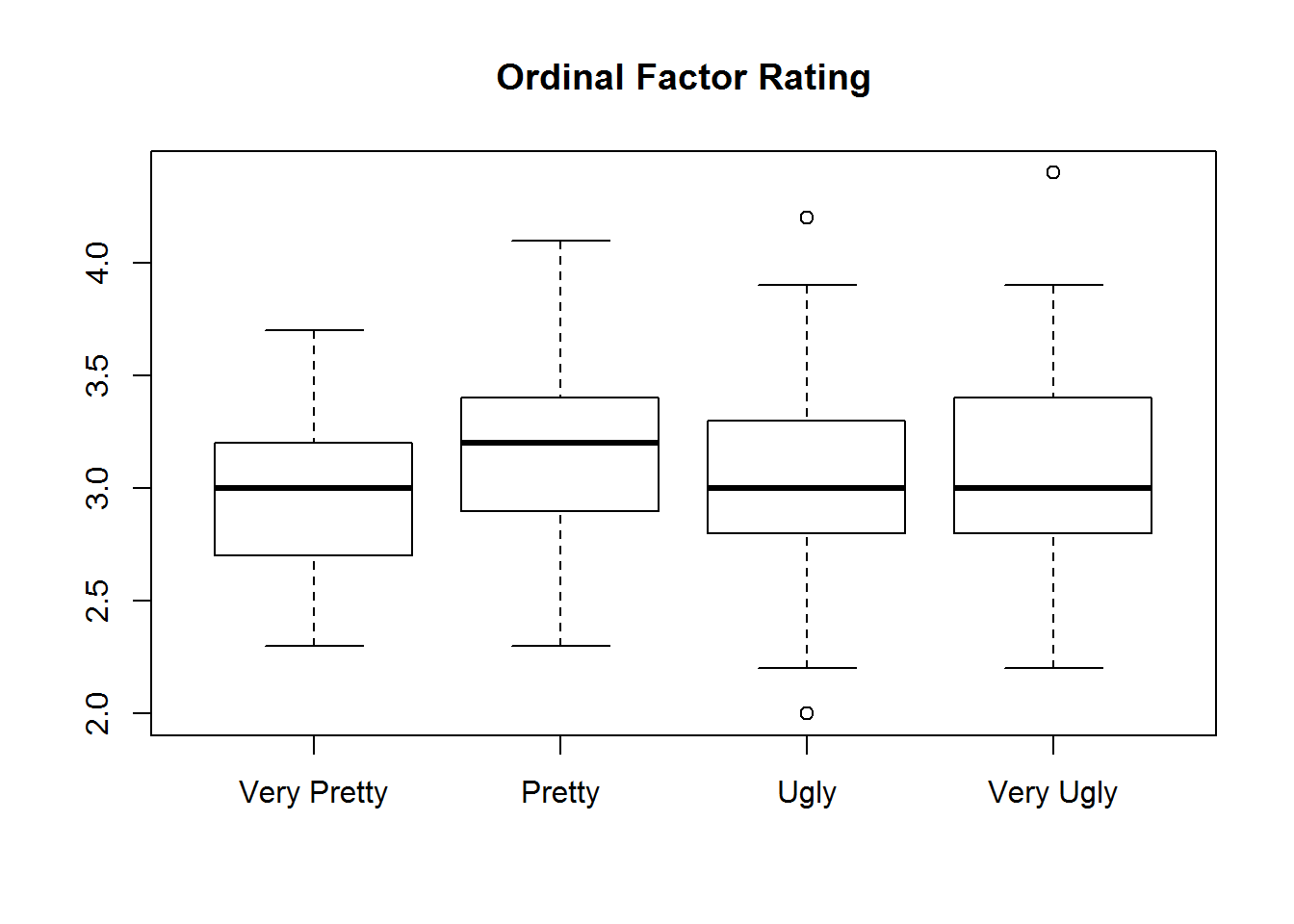
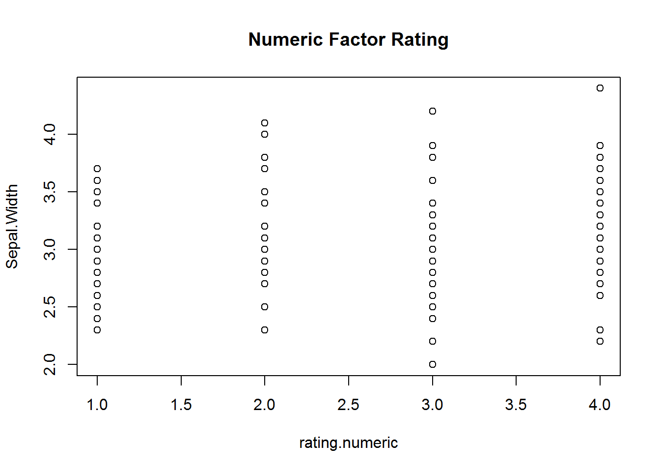
## $ rating.numeric: int 4 4 2 4 3 3 3 1 3 3 ...Here is a quick example of what this will look like when you try and use these for visualization or statistics.
with(iris, {
  plot(rating, Sepal.Width, main="Ordinal Factor Rating")
  plot(rating.numeric, Sepal.Width, main="Numeric Factor Rating")
})
Importing a Dataset
Create a folder close to root for use I usually use something like E:/Rcourse/L1. You can have R create the directory for you easily.
dir.create("E:/Rcourse/L1", showWarnings = FALSE)Then set the working directory for R to that folder. This lets you import and use the file easier. It also lets you know where to look for old workspaces and anything created by R (like a save file). I strongly – STRONGLY – recommend that you create a new directory for every analysis. Keep your original data in pristine format and have a syntax file that cleans the data and saves it to a new directory. Then when you do a primary analysis load that cleaned data and save any modification you make to a new directory. This allows you to go back to previous steps and easily make modifications without having to start over from the very beginning. It also means you will never have to admit you lost data, overwrote data, or in general screwed up. Computers have essentially unlimited data storage when used for typical social science research (a million rows of 30 variables stored in RData format is probably going to be less than 25 megabytes)
setwd("E:/Rcourse/L1")Text
A delimited file is always the best way to import data into R I would suggest exporting from SAS, SPSS, Excel, Etc. as a CSV then importing. We can even download a file from the internet if we know where to look for it. Here we can pull some responses to a Job in General survey
JiG <- read.csv(file = "http://degovx.eurybia.feralhosting.com/JiG.csv",
                fileEncoding = "UTF-8-BOM")
Most windows programs write a special bit of text at the front of text based files called a Byte Order Mark which can cause a bit of garbage to appear in the string of the first variable in the header. If you pass the fileEncoding BOM statement it cleans up that mark.
head(JiG)## XJIG1 XJIG2 XJIG3 XJIG4 XJIG5 XJIG6 XJIG7 XJIG8 XJIG9 XJIG10 XJIG11
## 1 3 3 3 3 3 3 3 3 3 3 3
## 2 3 3 1 3 3 3 3 3 3 0 3
## 3 3 3 3 3 3 3 3 3 3 0 0
## 4 3 3 0 3 3 3 3 3 3 0 0
## 5 3 3 3 3 3 3 3 3 3 3 3
## 6 3 3 3 3 3 3 3 3 3 0 3
## XJIG12 XJIG13 XJIG14 XJIG15 XJIG16 XJIG17 XJIG18 XJIG19x XJIG20x XJIG21x
## 1 3 3 3 3 3 3 3 3 3 3
## 2 3 3 3 0 3 3 3 3 3 3
## 3 3 3 3 0 3 3 3 3 3 0
## 4 3 0 3 0 3 3 3 0 3 0
## 5 3 3 3 3 3 3 3 3 3 3
## 6 3 3 3 3 3 3 3 3 3 3summary(JiG)## XJIG1 XJIG2 XJIG3 XJIG4
## Min. :0.000 Min. :0.000 Min. :0.000 Min. :0.000
## 1st Qu.:3.000 1st Qu.:3.000 1st Qu.:0.000 1st Qu.:3.000
## Median :3.000 Median :3.000 Median :0.000 Median :3.000
## Mean :2.488 Mean :2.699 Mean :1.092 Mean :2.663
## 3rd Qu.:3.000 3rd Qu.:3.000 3rd Qu.:3.000 3rd Qu.:3.000
## Max. :3.000 Max. :3.000 Max. :3.000 Max. :3.000
## XJIG5 XJIG6 XJIG7 XJIG8
## Min. :0.000 Min. :0.000 Min. :0.000 Min. :0.000
## 1st Qu.:3.000 1st Qu.:3.000 1st Qu.:3.000 1st Qu.:3.000
## Median :3.000 Median :3.000 Median :3.000 Median :3.000
## Mean :2.527 Mean :2.577 Mean :2.321 Mean :2.746
## 3rd Qu.:3.000 3rd Qu.:3.000 3rd Qu.:3.000 3rd Qu.:3.000
## Max. :3.000 Max. :3.000 Max. :3.000 Max. :3.000
## XJIG9 XJIG10 XJIG11 XJIG12
## Min. :0.00 Min. :0.0000 Min. :0.000 Min. :0.000
## 1st Qu.:3.00 1st Qu.:0.0000 1st Qu.:0.000 1st Qu.:3.000
## Median :3.00 Median :0.0000 Median :3.000 Median :3.000
## Mean :2.76 Mean :0.9461 Mean :2.122 Mean :2.574
## 3rd Qu.:3.00 3rd Qu.:3.0000 3rd Qu.:3.000 3rd Qu.:3.000
## Max. :3.00 Max. :3.0000 Max. :3.000 Max. :3.000
## XJIG13 XJIG14 XJIG15 XJIG16
## Min. :0.000 Min. :0.000 Min. :0.000 Min. :0.00
## 1st Qu.:0.000 1st Qu.:3.000 1st Qu.:0.000 1st Qu.:3.00
## Median :3.000 Median :3.000 Median :0.000 Median :3.00
## Mean :1.832 Mean :2.382 Mean :1.119 Mean :2.78
## 3rd Qu.:3.000 3rd Qu.:3.000 3rd Qu.:3.000 3rd Qu.:3.00
## Max. :3.000 Max. :3.000 Max. :3.000 Max. :3.00
## XJIG17 XJIG18 XJIG19x XJIG20x
## Min. :0.000 Min. :0.000 Min. :0.00 Min. :0.000
## 1st Qu.:1.000 1st Qu.:3.000 1st Qu.:1.00 1st Qu.:1.000
## Median :3.000 Median :3.000 Median :3.00 Median :3.000
## Mean :2.184 Mean :2.679 Mean :2.27 Mean :2.224
## 3rd Qu.:3.000 3rd Qu.:3.000 3rd Qu.:3.00 3rd Qu.:3.000
## Max. :3.000 Max. :3.000 Max. :3.00 Max. :3.000
## XJIG21x
## Min. :0.000
## 1st Qu.:0.000
## Median :0.000
## Mean :1.283
## 3rd Qu.:3.000
## Max. :3.000str(JiG)## 'data.frame': 1485 obs. of 21 variables:
## $ XJIG1 : int 3 3 3 3 3 3 3 3 0 3 ...
## $ XJIG2 : int 3 3 3 3 3 3 3 3 3 3 ...
## $ XJIG3 : int 3 1 3 0 3 3 3 0 0 3 ...
## $ XJIG4 : int 3 3 3 3 3 3 3 3 3 3 ...
## $ XJIG5 : int 3 3 3 3 3 3 3 0 3 3 ...
## $ XJIG6 : int 3 3 3 3 3 3 3 3 3 3 ...
## $ XJIG7 : int 3 3 3 3 3 3 3 1 3 3 ...
## $ XJIG8 : int 3 3 3 3 3 3 3 3 3 3 ...
## $ XJIG9 : int 3 3 3 3 3 3 3 3 3 3 ...
## $ XJIG10 : int 3 0 0 0 3 0 3 0 0 1 ...
## $ XJIG11 : int 3 3 0 0 3 3 3 0 3 3 ...
## $ XJIG12 : int 3 3 3 3 3 3 3 1 3 3 ...
## $ XJIG13 : int 3 3 3 0 3 3 3 0 0 3 ...
## $ XJIG14 : int 3 3 3 3 3 3 3 1 3 3 ...
## $ XJIG15 : int 3 0 0 0 3 3 3 0 0 3 ...
## $ XJIG16 : int 3 3 3 3 3 3 3 3 3 3 ...
## $ XJIG17 : int 3 3 3 3 3 3 3 1 3 3 ...
## $ XJIG18 : int 3 3 3 3 3 3 3 3 3 3 ...
## $ XJIG19x: int 3 3 3 0 3 3 3 0 3 3 ...
## $ XJIG20x: int 3 3 3 3 3 3 3 1 3 3 ...
## $ XJIG21x: int 3 3 0 0 3 3 3 0 0 3 ...We can even open the dataset for interaction
# view(JiG)Excel
Excel is supported only on Windows with the package RODBC or xlsx
SPSS, Stata, SAS
Most statistical software packages are supported with the package foreign
mydataframe <- read.spss(“mydata.sav”, use.value.labels=TRUE)
mydataframe <- read.dta(“mydata.dta”)
mydataframe <- read.xport(“mydata.dta”)
We can save the file we just downloaded as an RData file
save(JiG, file = "JiG.RData")Or export it as a csv
write.csv(JiG, file = "JiG.csv")If you are going to continue using R I recommend keeping files in RData it’s faster and smaller.
file.info(c("JiG.csv", "JiG.RData"))## size isdir mode mtime ctime
## JiG.csv 73330 FALSE 666 2015-06-24 14:00:56 2015-06-23 16:55:48
## JiG.RData 7964 FALSE 666 2015-06-24 14:00:56 2015-06-23 16:55:48
## atime exe
## JiG.csv 2015-06-23 16:55:48 no
## JiG.RData 2015-06-23 16:55:48 noUsing knitR
For your labs and creating beautiful reports you will be creating a syntax file that can be run in it’s entirety to give all the answers. They should also include comments like this specifying what question the next block of syntax is designed to answer. Once you are done with your syntax block you will run it with knitR. You run knitR through File -> Knit and select HTML notebook. Later we will go over how to use knitR to make pretty reports.
Now that you have completed Lesson 1 why not give your new skills a test?
Lab 1: https://docs.google.com/document/d/1BhOOOHf3-PrFurB3ZbuLb70zpFtc_8hYKITnLN_It7E/edit?usp=sharing
Answers: https://drive.google.com/file/d/0BzzRhb-koTrLZHRIM25QRTdZSFU/view?usp=sharing
If you are having issues with the answers try downloading them and opening them in your browser of choice.