Part III: Intermediate Data Management

Lesson 3: Intermediate Data Management

Most of the time someone spends working on a data analysis problem will be getting the data into the program. This starts with reading in a file and turns into transforming variables, correcting mistakes, and sometimes redesigning the entire dataset (e.g., long to tall changes). In this module we will begin to talk about how we can manipulate data in R to be the form we want for the analyses we want to conduct.

We are going to begin working with an actual dataset that will hopefully be a little entertaining as well as informative. First, we set a working directory to save files, graphs, etc. into. We can also have R create directories for us Show warnings = FALSE ignores warnings telling us the directory already exists (if it does already exist)

dir.create("E:/Rcourse/L3", showWarnings = FALSE)

Then set as working directory

setwd("E:/Rcourse/L3")

The dataset we will be using is a from IMDB and Rotten Tomatoes. You can find and create your own dataset with these variables or use the one linked here. We can start off by saving the file to the directory we set in the setwd step.

download.file(“http://degovx.eurybia.feralhosting.com/movies.RData”, “orig_movies.RData”)

Note: Making directories close to a root or in a home directory (documents in Windows, home in Linux, and whatever the equivalent is on an Apple machine) will make things a little less messy. I tend to partition a drive for doing analyses that automatically backs up every couple of days.

Once we have saved our file we can load it with a simple load statement (for RData file). We will look at a few different types of loading formats over the rest of the course including csv and fixed widths. See lesson 1 for some examples of loading and how to get data from common statistical programs.

load("E:/Rcourse/L3/orig_movies.RData")

The first step is to see how the data looks and to see how R has imported the various variables. We can do that with head (first 6 rows), tail (last 6 rows), summary (variable names and quantiles, max, and NAs of numeric variables), and str (type of variables and examples of the first few rows from each variable)

head(movies)

##                    Title Year Appropriate Runtime                    Genre
## 1             Carmencita 1894   NOT RATED   1 min       Documentary, Short
## 2 Le clown et ses chiens 1892        <NA>    <NA>         Animation, Short
## 3         Pauvre Pierrot 1892        <NA>   4 min Animation, Comedy, Short
## 4            Un bon bock 1892        <NA>    <NA>         Animation, Short
## 5       Blacksmith Scene 1893     UNRATED   1 min                    Short
## 6      Chinese Opium Den 1894        <NA>   1 min                    Short
##           Released             Director Writer Metacritic imdbRating
## 1             <NA> William K.L. Dickson   <NA>         NA        5.9
## 2 October 28, 1892        Émile Reynaud   <NA>         NA        6.5
## 3 October 28, 1892        Émile Reynaud   <NA>         NA        6.7
## 4 October 28, 1892        Émile Reynaud   <NA>         NA        6.6
## 5     May 09, 1893 William K.L. Dickson   <NA>         NA        6.3
## 6 October 17, 1894 William K.L. Dickson   <NA>         NA        5.9
##   imdbVotes Language Country Awards rtomRating rtomMeter rtomVotes Fresh
## 1       982     <NA>     USA   <NA>         NA        NA        NA    NA
## 2       118     <NA>  France   <NA>         NA        NA        NA    NA
## 3       523     <NA>  France   <NA>         NA        NA        NA    NA
## 4        79     <NA>  France   <NA>         NA        NA        NA    NA
## 5      1134     <NA>     USA 1 win.         NA        NA        NA    NA
## 6        53  English     USA   <NA>         NA        NA        NA    NA
##   Rotten rtomUserMeter rtomUserRating rtomUserVotes BoxOffice
## 1     NA            NA             NA            NA      <NA>
## 2     NA            NA             NA            NA      <NA>
## 3     NA            NA             NA            NA      <NA>
## 4     NA           100            2.8           216      <NA>
## 5     NA            32            3.0           184      <NA>
## 6     NA            NA             NA            NA      <NA>

summary(movies)

##     Title               Year           Appropriate       
##  Length:548010      Length:548010      Length:548010     
##  Class :character   Class :character   Class :character  
##  Mode  :character   Mode  :character   Mode  :character  
##                                                          
##                                                          
##                                                          
##                                                          
##    Runtime             Genre             Released        
##  Length:548010      Length:548010      Length:548010     
##  Class :character   Class :character   Class :character  
##  Mode  :character   Mode  :character   Mode  :character  
##                                                          
##                                                          
##                                                          
##                                                          
##    Director            Writer            Metacritic       imdbRating    
##  Length:548010      Length:548010      Min.   :  1.0    Min.   : 1.00   
##  Class :character   Class :character   1st Qu.: 45.0    1st Qu.: 5.60   
##  Mode  :character   Mode  :character   Median : 58.0    Median : 6.60   
##                                        Mean   : 56.5    Mean   : 6.38   
##                                        3rd Qu.: 69.0    3rd Qu.: 7.30   
##                                        Max.   :100.0    Max.   :10.00   
##                                        NA's   :537880   NA's   :197639  
##    imdbVotes         Language           Country         
##  Min.   :      5   Length:548010      Length:548010     
##  1st Qu.:     11   Class :character   Class :character  
##  Median :     29   Mode  :character   Mode  :character  
##  Mean   :   1614                                        
##  3rd Qu.:    127                                        
##  Max.   :1465210                                        
##  NA's   :197640                                         
##     Awards            rtomRating       rtomMeter        rtomVotes     
##  Length:548010      Min.   : 0.0     Min.   :  0.0    Min.   :  1.0   
##  Class :character   1st Qu.: 5.0     1st Qu.: 40.0    1st Qu.:  6.0   
##  Mode  :character   Median : 6.2     Median : 67.0    Median : 14.0   
##                     Mean   : 6.0     Mean   : 61.6    Mean   : 34.8   
##                     3rd Qu.: 7.1     3rd Qu.: 86.0    3rd Qu.: 39.0   
##                     Max.   :10.0     Max.   :100.0    Max.   :328.0   
##                     NA's   :529206   NA's   :529017   NA's   :526140  
##      Fresh            Rotten       rtomUserMeter    rtomUserRating  
##  Min.   :  0.0    Min.   :  0.0    Min.   :  0.0    Min.   :0.0     
##  1st Qu.:  3.0    1st Qu.:  1.0    1st Qu.: 34.0    1st Qu.:2.2     
##  Median :  8.0    Median :  4.0    Median : 58.0    Median :3.1     
##  Mean   : 21.6    Mean   : 13.2    Mean   : 55.8    Mean   :2.6     
##  3rd Qu.: 24.0    3rd Qu.: 12.0    3rd Qu.: 79.0    3rd Qu.:3.6     
##  Max.   :311.0    Max.   :195.0    Max.   :100.0    Max.   :5.0     
##  NA's   :526140   NA's   :526140   NA's   :485854   NA's   :455274  
##  rtomUserVotes       BoxOffice        
##  Min.   :       0   Length:548010     
##  1st Qu.:       6   Class :character  
##  Median :      74   Mode  :character  
##  Mean   :   25271                     
##  3rd Qu.:     512                     
##  Max.   :35791395                     
##  NA's   :455131

str(movies)

## Classes 'tbl_df', 'tbl' and 'data.frame':    548010 obs. of  23 variables:
##  $ Title         : chr  "Carmencita" "Le clown et ses chiens" "Pauvre Pierrot" "Un bon bock" ...
##  $ Year          : chr  "1894" "1892" "1892" "1892" ...
##  $ Appropriate   : chr  "NOT RATED" NA NA NA ...
##  $ Runtime       : chr  "1 min" NA "4 min" NA ...
##  $ Genre         : chr  "Documentary, Short" "Animation, Short" "Animation, Comedy, Short" "Animation, Short" ...
##  $ Released      : chr  NA "October 28, 1892" "October 28, 1892" "October 28, 1892" ...
##  $ Director      : chr  "William K.L. Dickson" "Émile Reynaud" "Émile Reynaud" "Émile Reynaud" ...
##  $ Writer        : chr  NA NA NA NA ...
##  $ Metacritic    : int  NA NA NA NA NA NA NA NA NA NA ...
##  $ imdbRating    : num  5.9 6.5 6.7 6.6 6.3 5.9 5.5 5.9 4.9 6.9 ...
##  $ imdbVotes     : int  982 118 523 79 1134 53 365 967 60 3376 ...
##  $ Language      : chr  NA NA NA NA ...
##  $ Country       : chr  "USA" "France" "France" "France" ...
##  $ Awards        : chr  NA NA NA NA ...
##  $ rtomRating    : num  NA NA NA NA NA NA NA NA NA NA ...
##  $ rtomMeter     : int  NA NA NA NA NA NA NA NA NA NA ...
##  $ rtomVotes     : int  NA NA NA NA NA NA NA NA NA NA ...
##  $ Fresh         : int  NA NA NA NA NA NA NA NA NA NA ...
##  $ Rotten        : int  NA NA NA NA NA NA NA NA NA NA ...
##  $ rtomUserMeter : int  NA NA NA 100 32 NA NA NA NA NA ...
##  $ rtomUserRating: num  NA NA NA 2.8 3 NA NA NA NA 3.8 ...
##  $ rtomUserVotes : int  NA NA NA 216 184 NA NA NA NA 124 ...
##  $ BoxOffice     : chr  NA NA NA NA ...

If you would like to interactively look at your dataset you can use view view(movies)

The first thing you should ask yourself is “How does the data look?” Then you should ask yourself “Are there any obvious issues?” Finally, you will probably have to ask yourself. How do I solve these problems?

For this dataset I see quite a few issues. Runtime, Released, Year, BoxOffice, Awards, and Appropriate are character vectors. Year and Released should be date variables. Genre, and Language have multiple entries in some rows. Genre, Language, Appropriate, Awards, and Country should all be nominal factors. Like most data analysis sessions getting the data into a format that is easy to use will be the first step. Followed by creating any variables that you may need. Using this data we will cover the basic tools of restructuring a dataset. ##Recoding Variables

Whether you are looking for a median split (shudder), you want to reverse code a scale, or your advisor has insisted you catagorize a continuous variable (because you would never do that yourself right?) you can do that relatively easily with base-R functionality. Recoding into a new variable is also great practice for the referencing we learned in previous lessons.

Let’s start out by breaking IMDB ratings down into bad (1-4), average (5-7), and good (8-10).

We can do this moderately quickly but cumbersomely with base-R First we duplicate the data from imdbRating into a new variable.

movies$imdbrate_cat <- movies$imdbRating

Then we take that new variable and we use the referencing to subset the variable into a smaller piece. Basically, we are saying from the movies dataset take the variable ($) imdbrate_cat. Then, within that variable find all instances where that variable meets a certain criterion. In this case that criterion is a logical operator. There are a number of simple logical operators in r.

Some Logical Operators:

< less than
<= less than or equal to
> greater than
>= greater than or equal to
== exactly equal to
!= not equal to
!x Not x
x | y x OR y
x & y x AND y
isTRUE(x) test if X is TRUE

Behind the scenes R makes a vector of TRUE and FALSE statements for every row, then selects all the rows which equal TRUE. With that subset in mind we tell r to assign either “Good”, “Average”, or “Bad

movies$imdbrate_cat[movies$imdbrate_cat >= 8] <- "Good"
movies$imdbrate_cat[movies$imdbrate_cat > 4 & 
                      movies$imdbrate_cat < 8] <- "Average"
movies$imdbrate_cat[movies$imdbrate_cat <= 4] <- "Bad"

We can take a look at our catagorization with the table() function. Table creates a contingency table of counts of combinations of factor levels. See help(table) for more information.

table(movies$imdbrate_cat)

## 
## Average     Bad    Good 
##  289971   21960   38440

We should also summarize our new variable to see how it was created.

summary(movies$imdbrate_cat)

##    Length     Class      Mode 
##    548010 character character

It looks like this variable is still a character variable and needs to be transformed into a factor. See Lesson 1 if you don’t remember how.

movies$imdbrate_cat <- factor(movies$imdbrate_cat, ordered=TRUE, 
                              levels=c("Bad", "Average", "Good"))
summary(movies$imdbrate_cat)

##     Bad Average    Good    NA's 
##   21960  289971   38440  197639

For many simple subsets or recodes this functionality is good. However, when you want to recode a lot of catagories at once using a package can be helpful. The best package for recoding (among a lot of other useful features that we will be using in this class) is the Companion to Applied Regression package.

require("car") #If you don't have it already install.packages("car")

## Loading required package: car

We will be using the recode() function. For more help type ?car or ?recode

movies$imdbrate_cat <- NA

NA is missing data. R treats both numeric and character missing the same. you can find missing with is.na() and exclude missing with na.rm = TRUE or use listwise deletion with na.omit = TRUE

recode(variable, “character string of changes”, options) Here we are telling cat to recode imdb rating. We are giving it a character string that has a couple of commands that recode recognizes (hi and lo). For more information on the commands available for recode try help(recode). We are also telling it that the outcome of the recode should be a factor and that factor is ordinal by passing the levels argument. Levels works exactly like in the factor command in base-R.

movies$imdbrate_cat <- recode(movies$imdbRating, "8:hi='Good';lo:4='Bad';4:8='Average'", 
                              as.factor.result = TRUE, levels=c("Bad", "Average", "Good"))
summary(movies$imdbrate_cat)

##     Bad Average    Good    NA's 
##   21960  289971   38440  197639

Later when we learn the apply statement we will learn how to recode any number of variables quickly using recode or base-R.

For now, let’s unload the car package since we won’t be using it anymore in this lesson.

detach("package:car", unload = TRUE)

Renaming Variables

You can open an interactive window with fix() to rename or modify variables like you would in SPSS or Excel. However, I find the interactive window to be rather slow and clumsy to use for more than 1 or 2 variables at a time. There are ways to rename variables through base-R functionality but I find packages simplify things immensly. For this we will be using the package dplyr. We will be using this package extensively in the next data management section as well as through the rest of the course.

require(dplyr) # install.packages("dplyr")

## Loading required package: dplyr
## 
## Attaching package: 'dplyr'
## 
## The following objects are masked from 'package:stats':
## 
##     filter, lag
## 
## The following objects are masked from 'package:base':
## 
##     intersect, setdiff, setequal, union

As you can see a few objects are “masked” from “package:Stats”. This means that those commands (filer, lag, intersect, etc.) will now be interpreted by the dplyr package rather than by the base-R package “Stats.” Normally, this won’t be much of an issue for most users since a well built package won’t break any functionality. However, this may not always be the case. If you find something just stops working try unloading any packages that aren’t essential to what you are doing. It can be a good tactic to load a package, do what you need with it, and unload it. Particularly, when you see one package masks commands from another package you will usually find functionality of one or both of the packages will be compromised. Pay attention to this warnings and if you want to use one of the commands that is being masked look into how that new command works to make sure you aren’t accidently making errors that can hinder interpretation of your results later.

rename(dataset, new_variable_name = old_variable_name). Additional variables can be added seperated by a comma.

movies <- rename(movies, imdbRatingCatagory = imdbrate_cat)

Date Variables

We have a couple of date variables in the dataset that will need to have some work done on them but the released variable needs the most so let’s start there. First, let’s take a look at released.

summary(movies$Released)

##    Length     Class      Mode 
##    548010 character character

str(movies$Released)

##  chr [1:548010] NA "October 28, 1892" "October 28, 1892" ...

head(movies$Released)

## [1] NA                 "October 28, 1892" "October 28, 1892"
## [4] "October 28, 1892" "May 09, 1893"     "October 17, 1894"

We have a character variable with the form MMMM dd, yyyy and some missing data. To see how R works with character data try visualing the variable with plot(movies$Released)

Looks like a character variable is unplottable. You could try a few other commands but you would find that character variables are pretty useless for analysis purposes. Later, we will find some uses for character variables, but most of the time you will want to get variables in the form of a number or factor.

R lets us tell it how variables should be classified with as. For example as.date(), as.numeric(), as.vector(), as.data.frame(), as.logical(). We can also test typing with is. for example, is.date() or is.numeric().

Before we convert this character string into a date we should make sure our localization is set correctly. In this case the data are English United States format. If your computer isn’t set to that localization you will have a bad time dealing with these dates.

Luckily, we can set localizations eazily.

Sys.setlocale("LC_TIME", "English")

## [1] "English_United States.1252"

Let’s try setting this variable as a date

head(as.Date(movies$Released))

The R as.Date command is well scripted and can recognize most common date formats. Sometimes, like above, you might run into something a little strange or unusual and you might need to set the format yourself. You can do that pretty easily. R uses POSIX for conversion. To find the commands specific to your format try help(strptime).

Looking at the help file we can see that a full month written out is a %B while the day is %d and four digit year is %Y

Note: as.Date uses a standard representation of time which sets a specific second as reference and all dates and times are stored as the time since or before that point.

We can specify our format as well as overwriting the current variable by giving as.Date a character string with the exact format (including commas, slashes, and dashes). We can also specify the time zone if there are hours, minutes, seconds, etc. in the string.

movies$Released <- as.Date(movies$Released, "%B %d, %Y", tz = "UTC")

summary(movies$Released)

##         Min.      1st Qu.       Median         Mean      3rd Qu. 
## "1888-10-14" "1982-12-03" "2004-09-23" "1993-04-16" "2010-06-13" 
##         Max.         NA's 
## "2022-01-01"      "66665"

str(movies$Released)

##  Date[1:548010], format: NA "1892-10-28" "1892-10-28" "1892-10-28" "1893-05-09" ...

head(movies$Released)

## [1] NA           "1892-10-28" "1892-10-28" "1892-10-28" "1893-05-09"
## [6] "1894-10-17"

Now our file has an appropriate date variable. We can see from summary that we are dealing with movies as early as 1888 and as late as 2022 (projected movies).

We can create a quick graph to look at number of movies released over time

hist(movies$Released, breaks = 10, main="Histogram of Movie Release Dates", xlab="Release Year")

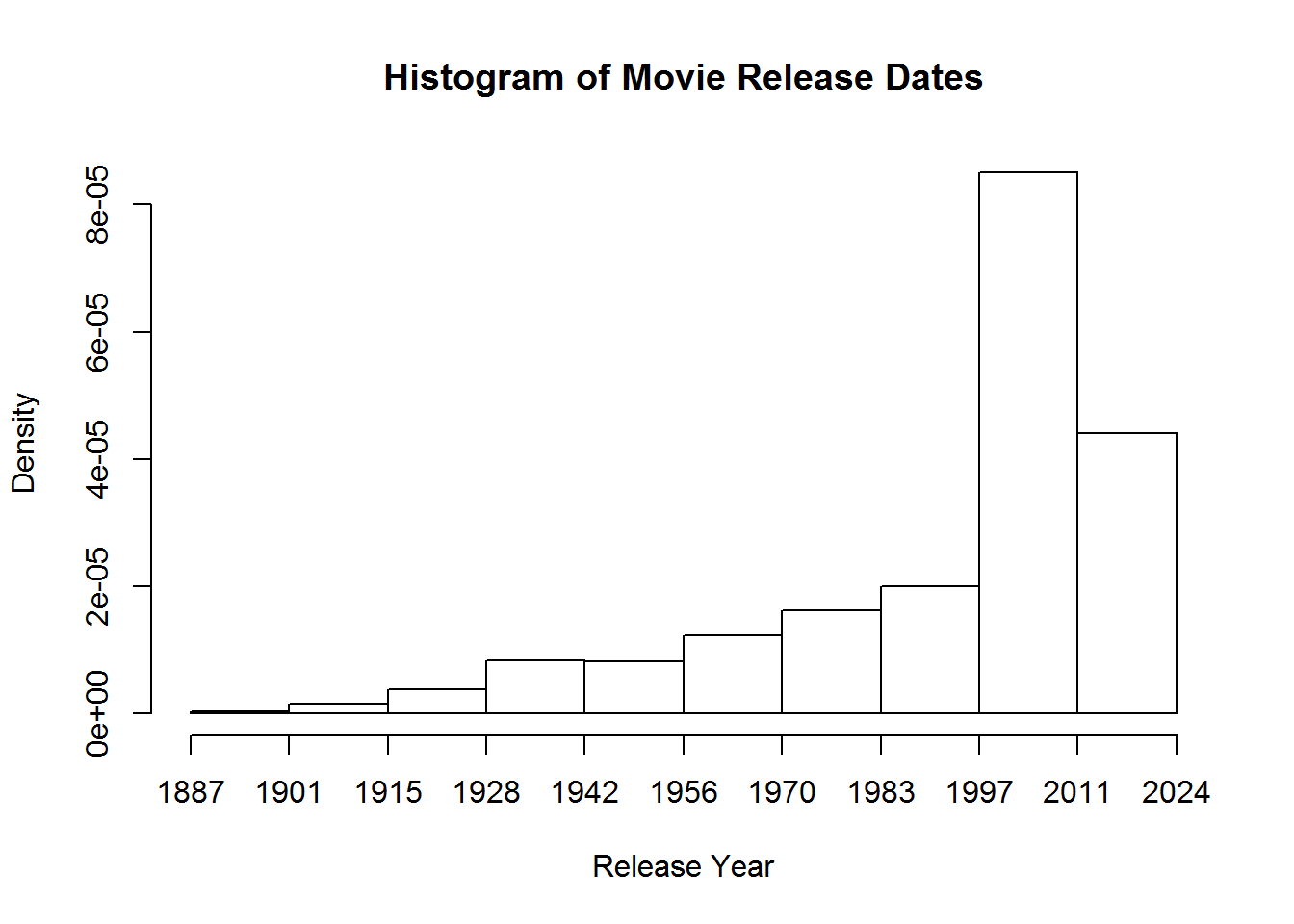
Using some of the fancy things we learned from last lesson we can put together a better graph. Let’s break it up so this histogram has a break for every year, change from density to frequency, and cut off the projected movies from the graph. We will have to specify that we want the x axis to be in years by using the as.Date command and format. Format will let us specify how we want the date represented. In this case, we want just years.

hist(movies$Released, breaks = (2015 - 1888), freq = TRUE, 
     main = "Histogram of Movie Release Dates", xlab = "Release Year",
     xlim = c(as.Date("1888", format="%Y"), as.Date("2015", format="%Y")))

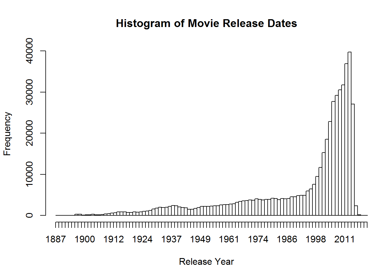
Regular Expressions in R

Now let’s convert Runtime to numeric. As we can see it’s a character vector still.

summary(movies$Runtime)

##    Length     Class      Mode 
##    548010 character character

str(movies$Runtime)

##  chr [1:548010] "1 min" NA "4 min" NA "1 min" "1 min" ...

head(movies$Runtime)

## [1] "1 min" NA      "4 min" NA      "1 min" "1 min"

We can try using the as.numberic statement like we did with as.Date

head(as.numeric(movies$Runtime))

## Warning in head(as.numeric(movies$Runtime)): NAs introduced by coercion

## [1] NA NA NA NA NA NA

Uhoh looks like R can’t handle that min in the string.

We can get around that by using pattern matching on the data. In this case we can use gsub (grep substitution of all matches using regular expressions) Use ?gsub for more information. Regular expressions are very powerful and spending some time learning how to use them will be a great benefit not only to R programming but any use of computers. You can learn a lot about regex from Wikipedia (https://en.wikipedia.org/wiki/Regular_expression) or from http://www.regular-expressions.info/tutorial.html

In this case we need only the most basic and simple search to accomplish our goals.

movies$Runtime <- as.numeric(gsub(" min", "", movies$Runtime))

## Warning: NAs introduced by coercion

summary(movies$Runtime)

##    Min. 1st Qu.  Median    Mean 3rd Qu.    Max.    NA's 
##    0.15   19.00   60.00   61.10   91.00  964.00   76827

str(movies$Runtime)

##  num [1:548010] 1 NA 4 NA 1 1 1 1 45 1 ...

head(movies$Runtime)

## [1]  1 NA  4 NA  1  1

Alright, we now have a usable variable. We can see we have movies from 15 seconds long to a little over 16 hours long. “Wait, what?” you are saying. 16 hour long movies? We can learn a bit about that exceptionally long movie fairly easily. We can find the maximum number with max() and remove NA’s from the analysis with na.rm = TRUE

max(movies$Runtime, na.rm = TRUE)

## [1] 964

Then all we have to do is look up that value. The easiest way to do that is to use which(). Which takes a logical vector (a vector of true and false statements) and returns the row number(s) that match the logic. Which is a useful function since it automatically allows NAs and sets them to FALSE. This is important because it gives an accurate return index. It’s a useful shortcut to a long statement.

movies[which(movies$Runtime == 964), ]

## Source: local data frame [1 x 24]
## 
##         Title  Year Appropriate Runtime                  Genre   Released
##         (chr) (chr)       (chr)   (dbl)                  (chr)     (date)
## 1 24 in Seven  2009          NA     964 Documentary, Adventure 2009-08-01
## Variables not shown: Director (chr), Writer (chr), Metacritic (int),
##   imdbRating (dbl), imdbVotes (int), Language (chr), Country (chr), Awards
##   (chr), rtomRating (dbl), rtomMeter (int), rtomVotes (int), Fresh (int),
##   Rotten (int), rtomUserMeter (int), rtomUserRating (dbl), rtomUserVotes
##   (int), BoxOffice (chr), imdbRatingCatagory (fctr)

“24 in Seven” is the long movie that doesn’t have any ratings. We can use which to find other things too. Like movies that are longer than 10 hours. Here we can use the index to select only titles and ratings.

movies[which(movies$Runtime > 600), c("Title", "imdbRating")]

## Source: local data frame [167 x 2]
## 
##                              Title imdbRating
##                              (chr)      (dbl)
## 1       Semnadtsat mgnoveniy vesny        9.1
## 2                      War & Peace        8.2
## 3                           Chlopi        7.2
## 4                      Noce i dnie        7.4
## 5                      I, Claudius        9.1
## 6   How Yukong Moved the Mountains        7.2
## 7                My Uncle Napoleon        8.6
## 8  Washington: Behind Closed Doors        8.0
## 9                 Die Buddenbrooks        8.1
## 10                       Flambards        8.3
## ..                             ...        ...

Let’s use our graphing skills again

hist(movies$Runtime, breaks = 100, main = "Histogram of Movie Runtimes", 
     xlab = "Runtime in Minutes")

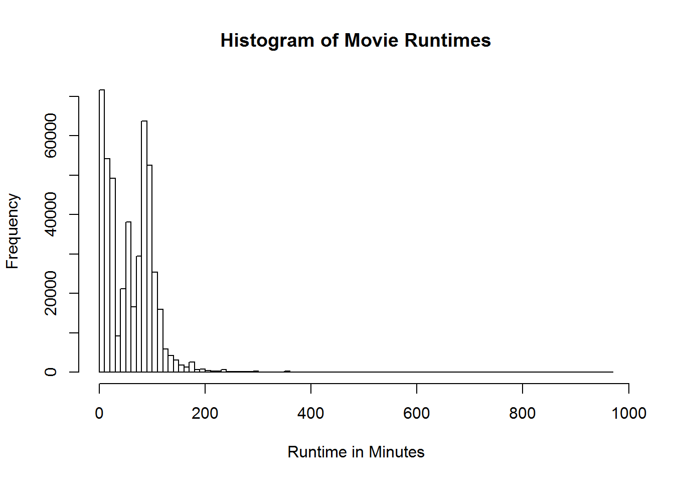
Those pesky outliers are making our graph pretty hard to read. Let’s drop down the graph to be movies that are just 5 hours or less. Before we just modified the graph to exclude those values. Let’s use the subsetting we learned to reduce the actual data being processed by the graph. This will generally be the prefered way since it speeds up the rest of the graphing process and takes less computational cycles.

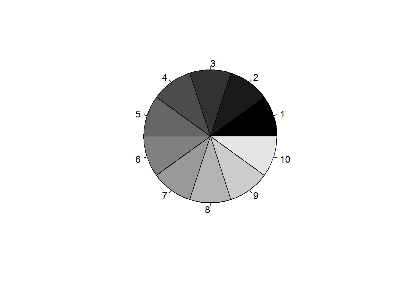
hist(movies$Runtime[movies$Runtime < 300], breaks = 100, 
     main = "Histogram of Movie Runtimes Excluding Outliers", 
     col = gray(0:100/100), xlab = "Runtime (Minutes)")

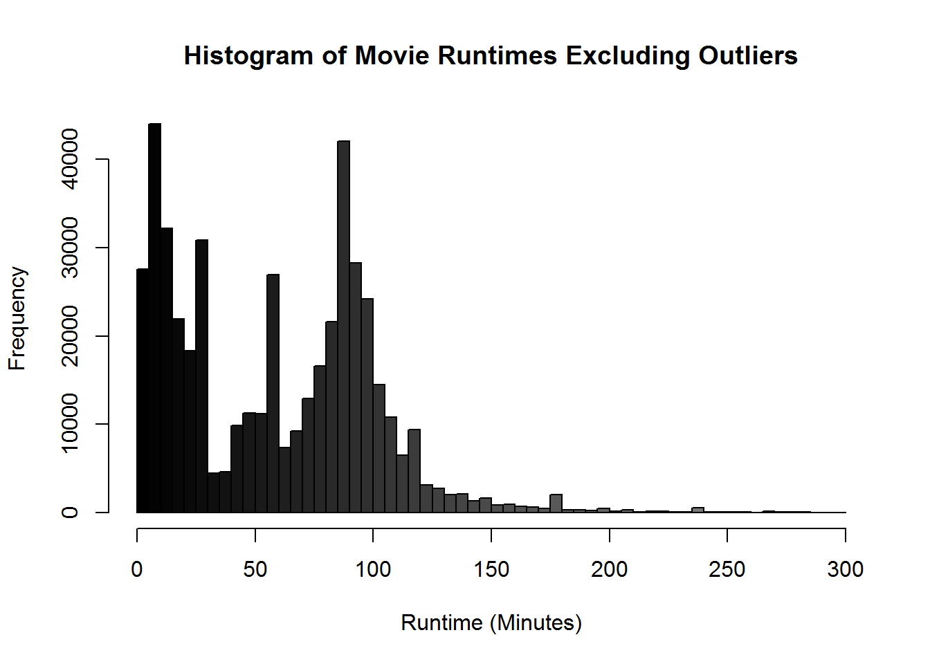
View the data again now that we have transformed it.

summary(movies)

##     Title               Year           Appropriate           Runtime      
##  Length:548010      Length:548010      Length:548010      Min.   :  0.15  
##  Class :character   Class :character   Class :character   1st Qu.: 19.00  
##  Mode  :character   Mode  :character   Mode  :character   Median : 60.00  
##                                                           Mean   : 61.10  
##                                                           3rd Qu.: 91.00  
##                                                           Max.   :964.00  
##                                                           NA's   :76827   
##     Genre              Released            Director        
##  Length:548010      Min.   :1888-10-14   Length:548010     
##  Class :character   1st Qu.:1982-12-03   Class :character  
##  Mode  :character   Median :2004-09-23   Mode  :character  
##                     Mean   :1993-04-16                     
##                     3rd Qu.:2010-06-13                     
##                     Max.   :2022-01-01                     
##                     NA's   :66665                          
##     Writer            Metacritic       imdbRating       imdbVotes      
##  Length:548010      Min.   :  1.0    Min.   : 1.00    Min.   :      5  
##  Class :character   1st Qu.: 45.0    1st Qu.: 5.60    1st Qu.:     11  
##  Mode  :character   Median : 58.0    Median : 6.60    Median :     29  
##                     Mean   : 56.5    Mean   : 6.38    Mean   :   1614  
##                     3rd Qu.: 69.0    3rd Qu.: 7.30    3rd Qu.:    127  
##                     Max.   :100.0    Max.   :10.00    Max.   :1465210  
##                     NA's   :537880   NA's   :197639   NA's   :197640   
##    Language           Country             Awards            rtomRating    
##  Length:548010      Length:548010      Length:548010      Min.   : 0.0    
##  Class :character   Class :character   Class :character   1st Qu.: 5.0    
##  Mode  :character   Mode  :character   Mode  :character   Median : 6.2    
##                                                           Mean   : 6.0    
##                                                           3rd Qu.: 7.1    
##                                                           Max.   :10.0    
##                                                           NA's   :529206  
##    rtomMeter        rtomVotes          Fresh            Rotten      
##  Min.   :  0.0    Min.   :  1.0    Min.   :  0.0    Min.   :  0.0   
##  1st Qu.: 40.0    1st Qu.:  6.0    1st Qu.:  3.0    1st Qu.:  1.0   
##  Median : 67.0    Median : 14.0    Median :  8.0    Median :  4.0   
##  Mean   : 61.6    Mean   : 34.8    Mean   : 21.6    Mean   : 13.2   
##  3rd Qu.: 86.0    3rd Qu.: 39.0    3rd Qu.: 24.0    3rd Qu.: 12.0   
##  Max.   :100.0    Max.   :328.0    Max.   :311.0    Max.   :195.0   
##  NA's   :529017   NA's   :526140   NA's   :526140   NA's   :526140  
##  rtomUserMeter    rtomUserRating   rtomUserVotes       BoxOffice        
##  Min.   :  0.0    Min.   :0.0      Min.   :       0   Length:548010     
##  1st Qu.: 34.0    1st Qu.:2.2      1st Qu.:       6   Class :character  
##  Median : 58.0    Median :3.1      Median :      74   Mode  :character  
##  Mean   : 55.8    Mean   :2.6      Mean   :   25271                     
##  3rd Qu.: 79.0    3rd Qu.:3.6      3rd Qu.:     512                     
##  Max.   :100.0    Max.   :5.0      Max.   :35791395                     
##  NA's   :485854   NA's   :455274   NA's   :455131                       
##  imdbRatingCatagory
##  Bad    : 21960    
##  Average:289971    
##  Good   : 38440    
##  NA's   :197639    
##                    
##                    
##

It looks like we still need to work on the variables Year, Appropriate, Genre, Director, Writer, Language, Country, Awards, and BoxOffice.

We will want to use Genre so let’s start there. First, we can use table to see a better summary of the data.

head(table(movies$Genre))

## 
##                   Action            Action, Adult Action, Adult, Adventure 
##                     4563                       14                        6 
## Action, Adult, Animation    Action, Adult, Comedy     Action, Adult, Crime 
##                        1                        8                        5

Here, with just head we can see that many catagories are present seperated by a comma. We could use regex to seperate these into new catagories but luckily for us there are already packages that can accomplish splitting, stacking, and shaping. Extra luckily for us these strings of combined information are constructed so the first entry is most important, second most, etc. That means we can take the first few catagories for each of these splits.

To accomplish the splitting we will be using tidyr. This is part of the family of packages like dplyr and plyr that we will be using in this course to manage data. Here we will be using a basic functionality to seperate a column of data into a number of new columns.

require(tidyr) # install.packages("tidyr")

## Loading required package: tidyr

the command we are interested in is separate(). separate(data, col, into, sep = “[^[:alnum:]]+”, remove = TRUE, convert = FALSE, extra = “error”, …)

For our purposes we are going to use the data movies, the column Genre, we want to make three new columns Genre_1, Genre_2, Genre_3, keep the original column in the data, split based on a comma, and drop any extra columns of data after three.

movies_genresplit <- separate(movies, Genre, c("Genre_1", "Genre_2", "Genre_3"), 
         remove = FALSE, sep = ",", extra = "drop")

tidyr is generally quick and easy but there are alternatives. A good alternative is the splitstackshape package which will automaticaly create a number of columns equal to the maximum number of splits. Splitstackshape uses the package data.table which we will not be covering in this course so once it has been used the resulting data needs to be converted back into a data frame before we can use it.

First, we will have to unload some packages since they conflict with splitstackshape

detach("package:dplyr", unload = TRUE)
detach("package:tidyr", unload = TRUE)

splitstackshape example

require("splitstackshape")

## Loading required package: splitstackshape
## Loading required package: data.table

movies <- cSplit(as.data.frame(movies), "Genre", sep=",")

setDF(movies)

summary(movies)

##     Title               Year           Appropriate           Runtime      
##  Length:548010      Length:548010      Length:548010      Min.   :  0.15  
##  Class :character   Class :character   Class :character   1st Qu.: 19.00  
##  Mode  :character   Mode  :character   Mode  :character   Median : 60.00  
##                                                           Mean   : 61.10  
##                                                           3rd Qu.: 91.00  
##                                                           Max.   :964.00  
##                                                           NA's   :76827   
##     Released            Director            Writer         
##  Min.   :1888-10-14   Length:548010      Length:548010     
##  1st Qu.:1982-12-03   Class :character   Class :character  
##  Median :2004-09-23   Mode  :character   Mode  :character  
##  Mean   :1993-04-16                                        
##  3rd Qu.:2010-06-13                                        
##  Max.   :2022-01-01                                        
##  NA's   :66665                                             
##    Metacritic       imdbRating       imdbVotes         Language        
##  Min.   :  1.0    Min.   : 1.00    Min.   :      5   Length:548010     
##  1st Qu.: 45.0    1st Qu.: 5.60    1st Qu.:     11   Class :character  
##  Median : 58.0    Median : 6.60    Median :     29   Mode  :character  
##  Mean   : 56.5    Mean   : 6.38    Mean   :   1614                     
##  3rd Qu.: 69.0    3rd Qu.: 7.30    3rd Qu.:    127                     
##  Max.   :100.0    Max.   :10.00    Max.   :1465210                     
##  NA's   :537880   NA's   :197639   NA's   :197640                      
##    Country             Awards            rtomRating       rtomMeter     
##  Length:548010      Length:548010      Min.   : 0.0     Min.   :  0.0   
##  Class :character   Class :character   1st Qu.: 5.0     1st Qu.: 40.0   
##  Mode  :character   Mode  :character   Median : 6.2     Median : 67.0   
##                                        Mean   : 6.0     Mean   : 61.6   
##                                        3rd Qu.: 7.1     3rd Qu.: 86.0   
##                                        Max.   :10.0     Max.   :100.0   
##                                        NA's   :529206   NA's   :529017  
##    rtomVotes          Fresh            Rotten       rtomUserMeter   
##  Min.   :  1.0    Min.   :  0.0    Min.   :  0.0    Min.   :  0.0   
##  1st Qu.:  6.0    1st Qu.:  3.0    1st Qu.:  1.0    1st Qu.: 34.0   
##  Median : 14.0    Median :  8.0    Median :  4.0    Median : 58.0   
##  Mean   : 34.8    Mean   : 21.6    Mean   : 13.2    Mean   : 55.8   
##  3rd Qu.: 39.0    3rd Qu.: 24.0    3rd Qu.: 12.0    3rd Qu.: 79.0   
##  Max.   :328.0    Max.   :311.0    Max.   :195.0    Max.   :100.0   
##  NA's   :526140   NA's   :526140   NA's   :526140   NA's   :485854  
##  rtomUserRating   rtomUserVotes       BoxOffice         imdbRatingCatagory
##  Min.   :0.0      Min.   :       0   Length:548010      Bad    : 21960    
##  1st Qu.:2.2      1st Qu.:       6   Class :character   Average:289971    
##  Median :3.1      Median :      74   Mode  :character   Good   : 38440    
##  Mean   :2.6      Mean   :   25271                      NA's   :197639    
##  3rd Qu.:3.6      3rd Qu.:     512                                        
##  Max.   :5.0      Max.   :35791395                                        
##  NA's   :455274   NA's   :455131                                          
##         Genre_1          Genre_2           Genre_3           Genre_4      
##  Short      :110902   Drama  : 62760   Drama   : 15207   Thriller:   269  
##  Documentary: 86989   Short  : 46557   Romance : 11662   Romance :   246  
##  Drama      : 81578   Comedy : 36044   Thriller:  9668   Family  :   200  
##  Comedy     : 74449   Romance: 14718   Comedy  :  7354   Drama   :   165  
##  Action     : 25638   Crime  :  9770   Family  :  6791   Fantasy :   151  
##  (Other)    :131529   (Other):102559   (Other) : 50743   (Other) :  1045  
##  NA's       : 36925   NA's   :275602   NA's    :446585   NA's    :545934  
##      Genre_5           Genre_6           Genre_7           Genre_8      
##  Thriller:    80   Thriller:    16   Sci-Fi  :     5   Music   :     1  
##  Romance :    52   Romance :    14   Thriller:     4   Musical :     1  
##  Sci-Fi  :    45   Sci-Fi  :     6   Music   :     2   Romance :     1  
##  War     :    40   Sport   :     6   War     :     2   Sci-Fi  :     1  
##  Fantasy :    33   Mystery :     5   Adult   :     1   Thriller:     4  
##  (Other) :   210   (Other) :    25   (Other) :     4   War     :     1  
##  NA's    :547550   NA's    :547938   NA's    :547992   NA's    :548001

Using either method we have sucessfully broken the Genre variable into multiple groups. Depending on which method we use we will have to do some cleanup. Using tidyr we would need to set the variables as factors since they are still strings. Using splitstackshape we can delete the extra columns that aren’t providing much information. For now, let’s use the output from splitstackshape and cover how to delete columns in R.

Subsetting a Dataset

It looks like we got 8 genre categories although the 4th genre only contains a handful of entries and the 8th only has 9. Let’s go ahead and delete the Genre_4 through 8. We can keep or drop variables a number of different ways.

Like we did above in the recoding section we can use dataframe element selection.

Since the extra columns are at the end of the dataset we can keep the beginning.

head(movies[, 1:26]) #We could just set this as movies with <-

##                    Title Year Appropriate Runtime   Released
## 1             Carmencita 1894   NOT RATED       1       <NA>
## 2 Le clown et ses chiens 1892        <NA>      NA 1892-10-28
## 3         Pauvre Pierrot 1892        <NA>       4 1892-10-28
## 4            Un bon bock 1892        <NA>      NA 1892-10-28
## 5       Blacksmith Scene 1893     UNRATED       1 1893-05-09
## 6      Chinese Opium Den 1894        <NA>       1 1894-10-17
##               Director Writer Metacritic imdbRating imdbVotes Language
## 1 William K.L. Dickson   <NA>         NA        5.9       982     <NA>
## 2        Émile Reynaud   <NA>         NA        6.5       118     <NA>
## 3        Émile Reynaud   <NA>         NA        6.7       523     <NA>
## 4        Émile Reynaud   <NA>         NA        6.6        79     <NA>
## 5 William K.L. Dickson   <NA>         NA        6.3      1134     <NA>
## 6 William K.L. Dickson   <NA>         NA        5.9        53  English
##   Country Awards rtomRating rtomMeter rtomVotes Fresh Rotten rtomUserMeter
## 1     USA   <NA>         NA        NA        NA    NA     NA            NA
## 2  France   <NA>         NA        NA        NA    NA     NA            NA
## 3  France   <NA>         NA        NA        NA    NA     NA            NA
## 4  France   <NA>         NA        NA        NA    NA     NA           100
## 5     USA 1 win.         NA        NA        NA    NA     NA            32
## 6     USA   <NA>         NA        NA        NA    NA     NA            NA
##   rtomUserRating rtomUserVotes BoxOffice imdbRatingCatagory     Genre_1
## 1             NA            NA      <NA>            Average Documentary
## 2             NA            NA      <NA>            Average   Animation
## 3             NA            NA      <NA>            Average   Animation
## 4            2.8           216      <NA>            Average   Animation
## 5            3.0           184      <NA>            Average       Short
## 6             NA            NA      <NA>            Average       Short
##   Genre_2 Genre_3
## 1   Short    <NA>
## 2   Short    <NA>
## 3  Comedy   Short
## 4   Short    <NA>
## 5    <NA>    <NA>
## 6    <NA>    <NA>

We could also refer to the entire string by name but that would be tedious. Instead let’s use the subset function. We can combine that with the through statement we learned earlier (:) to grab a range. NOTE: This doesn’t count up the numbers after the _ but selects the Genre_4 and Genre_8 and everything that is between the two of them in the dataset. Even things that don’t have Genre in the title. We will learn more later about how to select things that are counting up.

Subset works by giving a data location, then a logical statement for selecting rows, then select which tells which columns to use. If we give it no logical statement it assumes all rows and if give no column statements it assums all columns.

movies <- subset(movies, select = -(Genre_4:Genre_8))

Typical Genres

table(movies$Genre_1)

## 
##      Action       Adult   Adventure   Animation   Biography      Comedy 
##       25638       16260       10160       25101        4134       74449 
##       Crime Documentary       Drama      Family     Fantasy   Film-Noir 
##       13490       86989       81578        7988        1997          36 
##   Game-Show     History      Horror       Music     Musical     Mystery 
##        2101        1120        9673        7543        3126        2476 
##        News  Reality-TV     Romance      Sci-Fi       Short       Sport 
##        1576        5004        3347        2118      110902        2553 
##   Talk-Show    Thriller         War     Western 
##        2726        4885         763        3352

Subset is a very useful command that we will be using a bit in this class. We can easily use it to replicate a few of the logical statements we made earlier with a bit more ease.

Like selecting very long movies Before we used: movies[which(movies$Runtime > 600), c(“Title”, “imdbRating”)]

head(subset(movies, Runtime > 600, select = c("Title", "imdbRating")))

##                                Title imdbRating
## 51836     Semnadtsat mgnoveniy vesny        9.1
## 51860                    War & Peace        8.2
## 52050                         Chlopi        7.2
## 55075                    Noce i dnie        7.4
## 55513                    I, Claudius        9.1
## 55784 How Yukong Moved the Mountains        7.2

We can embed that subset into a statement to select rows for things like graphing. In this case we subset the data then use the $ to create a vector of just imdbRatings.

hist(subset(movies, Runtime > 600)$imdbRating, 
     main = "Histogram of IMDB Ratings for movies Over 600 Minutes",
     xlab = "IMDB ratings", xlim=c(1, 10), breaks = 10)

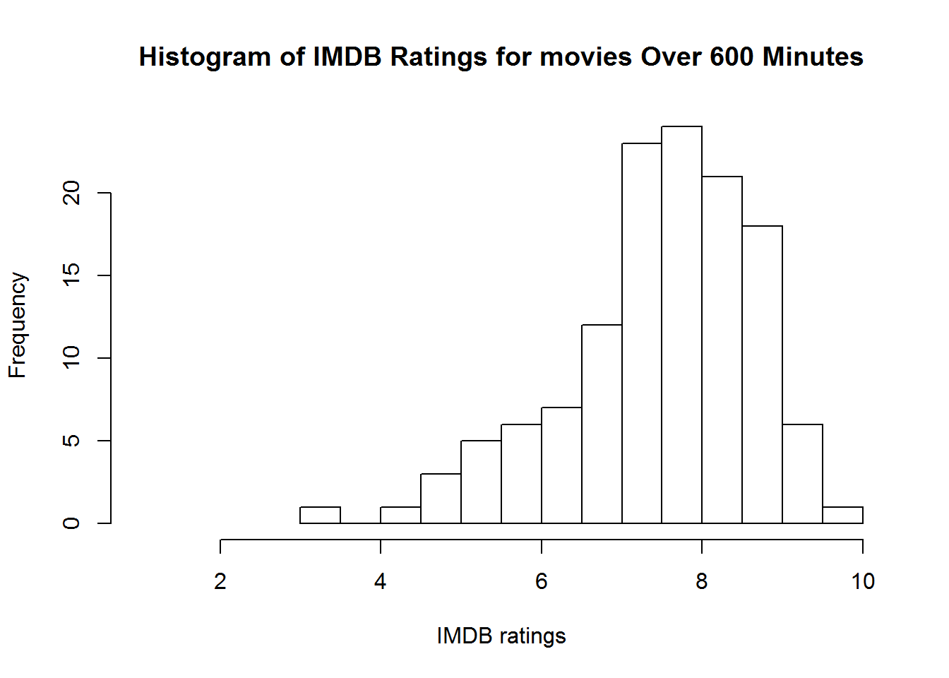
Now that we are experts on splitting and subsetting data let’s go ahead and tackle a couple of other variables. Why don’t you try and work through Language and Country yourselves before following along.

head(table(movies$Language))

## 
##                               Abkhazian 
##                                       2 
##                              Aboriginal 
##                                      16 
##                     Aboriginal, English 
##                                       5 
## Aboriginal, English, French, Portuguese 
##                                       1 
##           Aboriginal, Japanese, Hokkien 
##                                       1 
##         Aboriginal, Polynesian, English 
##                                       1

head(table(movies$Country))

## 
##                      Afghanistan              Afghanistan, France 
##                               21                                2 
## Afghanistan, France, Germany, UK                Afghanistan, Iran 
##                                1                                1 
##             Afghanistan, Ireland      Afghanistan, Ireland, Japan 
##                                1                                1

Like before these are long strings seperated by commas. Since we still have splitstackshape loaded I will use that again. One of the positives is that you can pass a character vector to cSplit to split multiple variables simultaneously.

movies <- cSplit(movies, c("Language","Country"), sep=",")
setDF(movies)

summary(movies)

##     Title               Year           Appropriate           Runtime      
##  Length:548010      Length:548010      Length:548010      Min.   :  0.15  
##  Class :character   Class :character   Class :character   1st Qu.: 19.00  
##  Mode  :character   Mode  :character   Mode  :character   Median : 60.00  
##                                                           Mean   : 61.10  
##                                                           3rd Qu.: 91.00  
##                                                           Max.   :964.00  
##                                                           NA's   :76827   
##     Released            Director            Writer         
##  Min.   :1888-10-14   Length:548010      Length:548010     
##  1st Qu.:1982-12-03   Class :character   Class :character  
##  Median :2004-09-23   Mode  :character   Mode  :character  
##  Mean   :1993-04-16                                        
##  3rd Qu.:2010-06-13                                        
##  Max.   :2022-01-01                                        
##  NA's   :66665                                             
##    Metacritic       imdbRating       imdbVotes          Awards         
##  Min.   :  1.0    Min.   : 1.00    Min.   :      5   Length:548010     
##  1st Qu.: 45.0    1st Qu.: 5.60    1st Qu.:     11   Class :character  
##  Median : 58.0    Median : 6.60    Median :     29   Mode  :character  
##  Mean   : 56.5    Mean   : 6.38    Mean   :   1614                     
##  3rd Qu.: 69.0    3rd Qu.: 7.30    3rd Qu.:    127                     
##  Max.   :100.0    Max.   :10.00    Max.   :1465210                     
##  NA's   :537880   NA's   :197639   NA's   :197640                      
##    rtomRating       rtomMeter        rtomVotes          Fresh       
##  Min.   : 0.0     Min.   :  0.0    Min.   :  1.0    Min.   :  0.0   
##  1st Qu.: 5.0     1st Qu.: 40.0    1st Qu.:  6.0    1st Qu.:  3.0   
##  Median : 6.2     Median : 67.0    Median : 14.0    Median :  8.0   
##  Mean   : 6.0     Mean   : 61.6    Mean   : 34.8    Mean   : 21.6   
##  3rd Qu.: 7.1     3rd Qu.: 86.0    3rd Qu.: 39.0    3rd Qu.: 24.0   
##  Max.   :10.0     Max.   :100.0    Max.   :328.0    Max.   :311.0   
##  NA's   :529206   NA's   :529017   NA's   :526140   NA's   :526140  
##      Rotten       rtomUserMeter    rtomUserRating   rtomUserVotes     
##  Min.   :  0.0    Min.   :  0.0    Min.   :0.0      Min.   :       0  
##  1st Qu.:  1.0    1st Qu.: 34.0    1st Qu.:2.2      1st Qu.:       6  
##  Median :  4.0    Median : 58.0    Median :3.1      Median :      74  
##  Mean   : 13.2    Mean   : 55.8    Mean   :2.6      Mean   :   25271  
##  3rd Qu.: 12.0    3rd Qu.: 79.0    3rd Qu.:3.6      3rd Qu.:     512  
##  Max.   :195.0    Max.   :100.0    Max.   :5.0      Max.   :35791395  
##  NA's   :526140   NA's   :485854   NA's   :455274   NA's   :455131    
##   BoxOffice         imdbRatingCatagory        Genre_1      
##  Length:548010      Bad    : 21960     Short      :110902  
##  Class :character   Average:289971     Documentary: 86989  
##  Mode  :character   Good   : 38440     Drama      : 81578  
##                     NA's   :197639     Comedy     : 74449  
##                                        Action     : 25638  
##                                        (Other)    :131529  
##                                        NA's       : 36925  
##     Genre_2           Genre_3         Language_01      Language_02    
##  Drama  : 62760   Drama   : 15207   English :274133   English:  7695  
##  Short  : 46557   Romance : 11662   German  : 28684   French :  3217  
##  Comedy : 36044   Thriller:  9668   Spanish : 27610   Spanish:  2834  
##  Romance: 14718   Comedy  :  7354   French  : 26076   German :  2366  
##  Crime  :  9770   Family  :  6791   Japanese: 18533   Tagalog:  1759  
##  (Other):102559   (Other) : 50743   (Other) :102686   (Other): 14433  
##  NA's   :275602   NA's    :446585   NA's    : 70288   NA's   :515706  
##   Language_03      Language_04      Language_05      Language_06    
##  English:  1881   English:   381   English:   112   German :    33  
##  French :   969   French :   307   French :    99   English:    32  
##  German :   828   German :   270   Spanish:    96   Spanish:    26  
##  Spanish:   590   Spanish:   203   German :    85   Italian:    24  
##  Italian:   443   Italian:   191   Italian:    75   Russian:    24  
##  (Other):  4148   (Other):  1525   (Other):   620   (Other):   218  
##  NA's   :539151   NA's   :545133   NA's   :546923   NA's   :547653  
##      Language_07         Language_08             Language_09    
##  Greek     :    17   Hebrew    :    10   Icelandic     :     9  
##  Russian   :    11   Portuguese:     7   Spanish       :     5  
##  Portuguese:    10   Italian   :     6   Italian       :     4  
##  Polish    :     9   Norwegian :     6   Russian       :     4  
##  English   :     7   Spanish   :     6   Serbo-Croatian:     4  
##  (Other)   :   110   (Other)   :    66   (Other)       :    43  
##  NA's      :547846   NA's      :547909   NA's          :547941  
##      Language_10             Language_11         Language_12    
##  Italian   :     9   Norwegian     :     8   Portuguese:     5  
##  Portuguese:     6   Spanish       :     5   Spanish   :     4  
##  Spanish   :     6   Swedish       :     5   French    :     3  
##  Polish    :     4   Portuguese    :     3   Polish    :     3  
##  Danish    :     3   Serbo-Croatian:     3   Italian   :     2  
##  (Other)   :    25   (Other)       :    21   (Other)   :    17  
##  NA's      :547957   NA's          :547965   NA's      :547976  
##          Language_13             Language_14             Language_15    
##  Portuguese    :     6   Serbo-Croatian:     4   Spanish       :     5  
##  Serbo-Croatian:     4   Spanish       :     4   Serbo-Croatian:     3  
##  Swedish       :     3   Turkish       :     4   Swedish       :     3  
##  Raeto-Romance :     2   Slovenian     :     3   German        :     1  
##  Slovak        :     2   Romanian      :     2   Hebrew        :     1  
##  (Other)       :     9   (Other)       :     7   (Other)       :     4  
##  NA's          :547984   NA's          :547986   NA's          :547993  
##     Language_16      Language_17        Language_18      Language_19    
##  Swedish  :     5   Turkish:     5   Bengali  :     1   Maltese:     1  
##  Turkish  :     3   Spanish:     2   Quechua  :     1   Russian:     1  
##  Slovenian:     2   Arabic :     1   Spanish  :     2   Swedish:     1  
##  Spanish  :     2   Finnish:     1   Swedish  :     2   Turkish:     2  
##  Arabic   :     1   Klingon:     1   Turkish  :     1   Uzbek  :     1  
##  (Other)  :     3   (Other):     3   Ukrainian:     1   NA's   :548004  
##  NA's     :547994   NA's   :547997   NA's     :548002                   
##   Language_20     Language_21    Language_22    Language_23   
##  Dutch  :     1   Mode:logical   Mode:logical   Mode:logical  
##  Turkish:     1   NA's:548010    NA's:548010    NA's:548010   
##  NA's   :548008                                               
##                                                               
##                                                               
##                                                               
##                                                               
##  Language_24    Language_25    Language_26    Language_27   
##  Mode:logical   Mode:logical   Mode:logical   Mode:logical  
##  NA's:548010    NA's:548010    NA's:548010    NA's:548010   
##                                                             
##                                                             
##                                                             
##                                                             
##                                                             
##    Country_01       Country_02       Country_03       Country_04    
##  USA    :202753   USA    :  6556   France :   949   France :   236  
##  UK     : 42264   France :  4579   USA    :   851   USA    :   213  
##  France : 25468   UK     :  2689   Germany:   732   Germany:   190  
##  Canada : 20137   Canada :  2526   UK     :   653   UK     :   179  
##  Japan  : 20082   Germany:  2389   Italy  :   449   Italy  :   144  
##  (Other):189691   (Other): 20353   (Other):  5030   (Other):  1694  
##  NA's   : 47615   NA's   :508918   NA's   :539346   NA's   :545354  
##    Country_05       Country_06           Country_07    
##  France :    83   Germany:    34   France     :    13  
##  USA    :    83   USA    :    34   Germany    :    13  
##  UK     :    77   France :    29   Netherlands:    12  
##  Germany:    64   Italy  :    26   UK         :    11  
##  Spain  :    36   UK     :    23   USA        :    11  
##  (Other):   664   (Other):   265   (Other)    :   171  
##  NA's   :547003   NA's   :547599   NA's       :547779  
##        Country_08       Country_09         Country_10    
##  Germany    :     9   France :     8   UK       :     4  
##  Austria    :     6   Canada :     5   Australia:     3  
##  France     :     6   Italy  :     5   Belgium  :     3  
##  Switzerland:     6   Belgium:     4   China    :     3  
##  UK         :     6   UK     :     4   Israel   :     3  
##  (Other)    :   123   (Other):    79   (Other)  :    55  
##  NA's       :547854   NA's   :547905   NA's     :547939  
##         Country_11       Country_12       Country_13       Country_14    
##  Hungary     :     4   Germany:     3   France :     5   Ecuador:     2  
##  Italy       :     4   China  :     2   India  :     2   Estonia:     2  
##  South Africa:     4   Egypt  :     2   Israel :     2   Germany:     2  
##  Finland     :     3   Ireland:     2   Mexico :     2   Russia :     2  
##  Canada      :     2   Italy  :     2   UK     :     2   Brazil :     1  
##  (Other)     :    40   (Other):    27   (Other):    16   (Other):    14  
##  NA's        :547953   NA's   :547972   NA's   :547981   NA's   :547987  
##    Country_15              Country_16                  Country_17    
##  Denmark:     3   Austria       :     2   Croatia           :     2  
##  Israel :     3   Czech Republic:     2   India             :     2  
##  Georgia:     2   Congo         :     1   China             :     1  
##  Japan  :     2   Côte d'Ivoire :     1   Czech Republic    :     1  
##  China  :     1   Ethiopia      :     1   Dominican Republic:     1  
##  (Other):     9   (Other)       :    11   (Other)           :     7  
##  NA's   :547990   NA's          :547992   NA's              :547996  
##     Country_18                      Country_19         Country_20    
##  Bulgaria:     2   Belgium               :     3   Austria  :     2  
##  Cambodia:     2   Bangladesh            :     1   Argentina:     1  
##  Brazil  :     1   Bosnia and Herzegovina:     1   Australia:     1  
##  Croatia :     1   Brazil                :     1   Belgium  :     1  
##  Germany :     1   France                :     1   Bolivia  :     1  
##  (Other) :     6   (Other)               :     6   (Other)  :     7  
##  NA's    :547997   NA's                  :547997   NA's     :547997  
##        Country_21         Country_22            Country_23    
##  Albania    :     1   Australia:     1   Argentina   :     1  
##  Bhutan     :     1   Canada   :     1   Belgium     :     1  
##  Chile      :     1   France   :     1   Egypt       :     1  
##  India      :     1   Russia   :     1   South Africa:     1  
##  Philippines:     1   Slovenia :     1   Spain       :     1  
##  (Other)    :     4   (Other)  :     2   (Other)     :     2  
##  NA's       :548001   NA's     :548003   NA's        :548003  
##           Country_24          Country_25        Country_26    
##  Australia     :     1   Antarctica:     1   Cambodia:     1  
##  Czech Republic:     1   China     :     1   NA's    :548009  
##  Sweden        :     1   Turkey    :     1                    
##  Syria         :     1   UK        :     1                    
##  Uruguay       :     1   NA's      :548006                    
##  NA's          :548005                                        
##                                                               
##      Country_27    
##  Australia:     1  
##  NA's     :548009  
##                    
##                    
##                    
##                    
##

Like before we will also need to deal with all these extra columns. Many of which don’t have much information contained within.

movies <- subset(movies, select = -(Language_04:Language_27))
movies <- subset(movies, select = -(Country_04:Country_27))

Now that we have divided up language and country why don’t we see how many Turkish movies Are in this list. We also want to find out something about how good the movies are so let’s select movies that don’t have missing data for IMDb Ratings. Here we can combine what we have learned before to create a powerful search of the data to create a subset.

TurkishMovies <- subset(movies, Country_01=="Turkey" & 
                          Language_01=="Turkish" &
                          !is.na(imdbRating), 
                        select=c("Title", "imdbRating"))
head(TurkishMovies, n = 10)

##                                                        Title imdbRating
## 13528                              Aysel: Batakli damin kizi        7.1
## 45280                                   O Beautiful Istanbul        8.2
## 45503                                             Dry Summer        8.0
## 45856                                       Atesli delikanli        5.2
## 49119                                                   Hope        8.2
## 49374 Little Ayse and the Magic Dwarfs in the Land of Dreams        5.0
## 50333                                             Umutsuzlar        7.3
## 50583                                                   Agit        7.1
## 51942                                                   Baba        7.3
## 52237                                                  Gelin        7.8

So what are the best and the worst Turkish movies? We can use order to arrange our dataset and head to display just the top and tail to display the bottom

TurkishMovies <- TurkishMovies[order(-TurkishMovies$imdbRating, TurkishMovies$Title), ]

head(TurkishMovies)

##                         Title imdbRating
## 153141        The Chaos Class        9.5
## 480119 CM101MMXI Fundamentals        9.4
## 480973 CM101MMXI Fundamentals        9.4
## 377955           C.M.Y.L.M.Z.        9.3
## 533766            Kardes Payi        9.3
## 213335       Bir Tat Bir Doku        9.2

tail(TurkishMovies)

##                                Title imdbRating
## 461030                   Hep ezildim        1.8
## 410372               Kahkaha Marketi        1.8
## 254248 Keloglan vs. the Black Prince        1.8
## 329286                Super Agent K9        1.4
## 298894              Yildizlar savasi        1.2
## 529115                       Tersine        1.0

It seems our dataset contains at least a few duplicated rows. For instance here we can see CM101MMXI Fundamentals seems to be so good it was included twice. We can verify that is in fact a duplicate by looking at it.

movies[c(480119, 480973), ]

##                         Title Year Appropriate Runtime   Released
## 480119 CM101MMXI Fundamentals 2013        <NA>     139 2013-01-03
## 480973 CM101MMXI Fundamentals 2013        <NA>     139 2013-01-03
##            Director     Writer Metacritic imdbRating imdbVotes Awards
## 480119 Murat Dundar Cem Yilmaz         NA        9.4     32992   <NA>
## 480973 Murat Dundar Cem Yilmaz         NA        9.4     32161   <NA>
##        rtomRating rtomMeter rtomVotes Fresh Rotten rtomUserMeter
## 480119         NA        NA        NA    NA     NA            NA
## 480973         NA        NA        NA    NA     NA            NA
##        rtomUserRating rtomUserVotes BoxOffice imdbRatingCatagory
## 480119             NA            NA      <NA>               Good
## 480973             NA            NA      <NA>               Good
##            Genre_1 Genre_2 Genre_3 Language_01 Language_02 Language_03
## 480119 Documentary  Comedy    <NA>     Turkish        <NA>        <NA>
## 480973 Documentary  Comedy    <NA>     Turkish        <NA>        <NA>
##        Country_01 Country_02 Country_03
## 480119     Turkey       <NA>       <NA>
## 480973     Turkey       <NA>       <NA>

Finding duplicate rows can be tedious in a small dataset. In a dataset with over 500k observations it’s impossible to do manually. R has a couple of ways to identify unique and duplicate cases.

The easiest is duplicated(dataframe) which looks for two rows that are exactly the same. This will identify many duplicates but not ones with even superficial differences. For example, CM101MMXI Fundamentals has different numbers of votes in the imdbVotes variable so it wouldn’t be identified as a duplicate. It will also assume that the first row in the dataset is the original unless fromLast = TRUE. Finally, it is not the fastest operation. We can have it run a bit quicker by getting rid of movies that have the same Title but it will remove movies that are actually different that happen to have the same title. How you manage duplicates is up to you, for the purposes of this dataset a conservative approach is best since it’s likely many movies share a title.

We can save this as two data frames. One with the duplicated movies and the second is our movies dataframe with the duplicates removed.

duplicated_movies <- movies[duplicated(movies), ]

movies <- movies[!duplicated(movies), ]

Exporting a File

Alright now let’s export this file so we can use it in later projects. It’s good data management to create new files after modifying your data so you can go back to previous versions or to store each iteration of your data in a new folder. Always preserve your original data without modifications. You have all the syntax here in R so you can easily re-run a syntax file partially to correct errors. It’s never that easy to recover missing, destroyed, or incorrectly modified data.

New Folder Method

At the beginning on the lesson we created a folder and set our working directory to that folder. Then we downloaded our file and called it movies_orig.RData. As long as we don’t overwrite that file we will have our original data. I prefer this method myself because I like folder based organization. Usually, I name my folders with the project name followed by the date I am working.

save(data, list of objects to save, file to save them in)

For example, we could save everything into an RData file with:

save(movies, file="movies.RData")

or as a csv with

write.table(movies, file="movies.csv", sep=",")

If you are going to continue using R I recommend keeping files in RData it’s faster and smaller.

file.info(c("movies.csv", "movies.RData"))

##                   size isdir mode               mtime               ctime
## movies.csv   107340331 FALSE  666 2015-09-10 12:10:46 2015-09-09 15:12:51
## movies.RData  25541925 FALSE  666 2015-09-10 12:10:27 2015-09-09 15:12:43
##                            atime exe
## movies.csv   2015-09-09 15:12:51  no
## movies.RData 2015-09-09 15:12:43  no

Automatic Naming of Data Files

We can use R to automatically generate these saves in an easy to preserve format. We combine the paste which we have used before with the same command and a new command Sys.Date() which looks to your computer to find what today’s date is. This can be modified to include the hour, minute, or second to make completely sure every time you save a file it generates a new one. I find that having the day in front of the file is frequently good enough.

save(movies, file = paste(Sys.Date(), "movies.RData", sep=" "))

Let’s test out our knowledge of cleaning a dataset with lab 3. You can download it here: https://docs.google.com/document/d/17MFukYodljz6nIdgJIvS-G_g6B11nHcvZmsf4yhiP4M/edit?usp=sharing

Answers: https://drive.google.com/file/d/0BzzRhb-koTrLNWJsT2N4ZTAtU0U/view?usp=sharing

If you are having issues with the answers try downloading them and opening them in your browser of choice.

Part II: Introduction to Base-R Graphing

Here we begin the journey that is graphing with R. The ability to make beautiful and compelling graphs quickly was what drew me into using R in the first place. Later, I began to use graphing packages like ggplot2 and ggvis and quickly found that making high quality and publishable plots is easy. Perhaps one of the most exciting (and new) features of R is the introduction of packages like shiny which allow for direct translation of R code into javascript code. Later we will be exploring some of these exciting uses of R. Particularly, we will focus on how to make an interactive report where someone can drag a slider bar around to adjust aspects of your graph. A sure sign that you are bound for promotion!

Graphing in R is very powerful. Think of graphing in R as a construction project. We start by laying down a foundation (specifying the data), then we build the framework (specifying the axes, labeling, titling, etc.), then we fill in the rest of the structure with the walls and details (specifying the statistics that are displayed in the graph). Base-R has a large suite of tools for graphing and does a commendable job quickly plotting what researchers need to see. The tools exist to build a plot that you desire but many turn to packages for true graphing freedom. The most propular packages are lattice and ggplot2 with the sucessor to ggplot2, ggvis, gaining in popularity. We will later be covering ggplot2 since it is more refined and less subject to change than ggvis.

We will work with one of the R learning dataframes today. The data was extracted from the 1974 Motor Trend US magazine, and comprises fuel consumption and 10 aspects of automobile design and performance for 32 automobiles (1973-74 models)

head(mtcars)

##                    mpg cyl disp  hp drat    wt  qsec vs am gear carb
## Mazda RX4         21.0   6  160 110 3.90 2.620 16.46  0  1    4    4
## Mazda RX4 Wag     21.0   6  160 110 3.90 2.875 17.02  0  1    4    4
## Datsun 710        22.8   4  108  93 3.85 2.320 18.61  1  1    4    1
## Hornet 4 Drive    21.4   6  258 110 3.08 3.215 19.44  1  0    3    1
## Hornet Sportabout 18.7   8  360 175 3.15 3.440 17.02  0  0    3    2
## Valiant           18.1   6  225 105 2.76 3.460 20.22  1  0    3    1

summary(mtcars)

##       mpg             cyl             disp             hp       
##  Min.   :10.40   Min.   :4.000   Min.   : 71.1   Min.   : 52.0  
##  1st Qu.:15.43   1st Qu.:4.000   1st Qu.:120.8   1st Qu.: 96.5  
##  Median :19.20   Median :6.000   Median :196.3   Median :123.0  
##  Mean   :20.09   Mean   :6.188   Mean   :230.7   Mean   :146.7  
##  3rd Qu.:22.80   3rd Qu.:8.000   3rd Qu.:326.0   3rd Qu.:180.0  
##  Max.   :33.90   Max.   :8.000   Max.   :472.0   Max.   :335.0  
##       drat             wt             qsec             vs        
##  Min.   :2.760   Min.   :1.513   Min.   :14.50   Min.   :0.0000  
##  1st Qu.:3.080   1st Qu.:2.581   1st Qu.:16.89   1st Qu.:0.0000  
##  Median :3.695   Median :3.325   Median :17.71   Median :0.0000  
##  Mean   :3.597   Mean   :3.217   Mean   :17.85   Mean   :0.4375  
##  3rd Qu.:3.920   3rd Qu.:3.610   3rd Qu.:18.90   3rd Qu.:1.0000  
##  Max.   :4.930   Max.   :5.424   Max.   :22.90   Max.   :1.0000  
##        am              gear            carb      
##  Min.   :0.0000   Min.   :3.000   Min.   :1.000  
##  1st Qu.:0.0000   1st Qu.:3.000   1st Qu.:2.000  
##  Median :0.0000   Median :4.000   Median :2.000  
##  Mean   :0.4062   Mean   :3.688   Mean   :2.812  
##  3rd Qu.:1.0000   3rd Qu.:4.000   3rd Qu.:4.000  
##  Max.   :1.0000   Max.   :5.000   Max.   :8.000

str(mtcars)

## 'data.frame':    32 obs. of  11 variables:
##  $ mpg : num  21 21 22.8 21.4 18.7 18.1 14.3 24.4 22.8 19.2 ...
##  $ cyl : num  6 6 4 6 8 6 8 4 4 6 ...
##  $ disp: num  160 160 108 258 360 ...
##  $ hp  : num  110 110 93 110 175 105 245 62 95 123 ...
##  $ drat: num  3.9 3.9 3.85 3.08 3.15 2.76 3.21 3.69 3.92 3.92 ...
##  $ wt  : num  2.62 2.88 2.32 3.21 3.44 ...
##  $ qsec: num  16.5 17 18.6 19.4 17 ...
##  $ vs  : num  0 0 1 1 0 1 0 1 1 1 ...
##  $ am  : num  1 1 1 0 0 0 0 0 0 0 ...
##  $ gear: num  4 4 4 3 3 3 3 4 4 4 ...
##  $ carb: num  4 4 1 1 2 1 4 2 2 4 ...

help(mtcars) for more info on the dataset.

This is an American dataset so we can convert to metric for measurements that make sense. Like we did in lesson 1 we use within to state which dataframe to use (in this case mtcars). Then we use a curly bracket to frame what we want to manipulate. The curly brackets help keep the syntax organized. At the end we assign the data back to the mtcars datafame with a right facing arrow.

within(mtcars, {
  kpl <- mpg * 0.425
  wt.mt <- wt * 0.454
  disp.c <- disp * 2.54
}) -> mtcars

The Most Basic Graph

First we lay the foundation

Graph weight by kilometers per liter.
We are using the mtcars dataframe and some variables that are in that dataframe. Like in lesson 1 we need to tell R what dataframe the variables are in. We do that by using the $. mtcars is the data and WITHIN ($) that data is the variable wt.mt.
Then we overlay that foundation with a least squares line.
abline = straight line graphic
lm = linear model
~ is the by command here we are saying graph kpl by wt.ml

plot(mtcars$wt.mt, mtcars$kpl)
abline(lm(mtcars$kpl ~ mtcars$wt.mt))
title("Regression of Kilometers per Liter on Weight in Metric Tons")

Now let’s put some strucural components in place

Saving a Graph to the Hard Drive

I am too lazy to make a folder so let’s have R do it for us.

dir.create("E:/Rcourse/L2", showWarnings = FALSE)

Make that new folder the working directory.

setwd("E:/Rcourse/L2")

Let’s take the commands above and create a file instead of displaying.
First we need to tell what engine to use. I prefer png since it’s a good mix of compression and quality. You can specify pdf or tiff for good lossless saves, jpg for small and low quality, or bmp, xfig, and postscript for embedding or modifications. Just be sure that whatever engine you specify you also specify a file extention that matches.
This will start a graphical device (dev) which saves console output to that device until it ends with dev.off(). You could use this to capture table output or anything else you like.

png("graph1.png")
plot(mtcars$wt.mt, mtcars$kpl)
abline(lm(mtcars$kpl ~ mtcars$wt.mt))
title("Regression of Kilometers per Liter on Weight in Metric Tons")
dev.off()

## png 
##   2

Notice nothing is generated in the plot window.
You can specify the size of the graph in the dev with width, height, and units. You can also specify plotted point size with pointsize, background with bg, resolution in ppi with res, and depending on the file type some measure of quality or compression type. See ?png or ?pdf for more information.

png("graph2.png", width = 1000, height = 806, units = "px", res = 150)
plot(mtcars$wt.mt, mtcars$kpl)
abline(lm(mtcars$kpl ~ mtcars$wt.mt))
title("Regression of Kilometers per Liter on Weight in Metric Tons")
dev.off()

## png 
##   2

Here we are specifying a graph that is 1000 by 806 pixels and adjusting res so the graph isn’t tiny at that size

If you have been saving images and suddenly your commands don’t seem to be doing anything anymore it’s probably because a dev is still running. You can simply run dev.off() until R prints null device 1 or gives the error “cannot shut down device 1”

R studio also support saving a graph through the point and click menus. Check the export box and modify settings accordingly.

Making Graphs Pretty and Functional

R controls graph displays with graphical parameters or par(). They function as par(optionname=VALUE, optionname=VALUE)

par(no.readonly=TRUE) #These are all the parameters you can manipulate.

## $xlog
## [1] FALSE
## 
## $ylog
## [1] FALSE
## 
## $adj
## [1] 0.5
## 
## $ann
## [1] TRUE
## 
## $ask
## [1] FALSE
## 
## $bg
## [1] "white"
## 
## $bty
## [1] "o"
## 
## $cex
## [1] 1
## 
## $cex.axis
## [1] 1
## 
## $cex.lab
## [1] 1
## 
## $cex.main
## [1] 1.2
## 
## $cex.sub
## [1] 1
## 
## $col
## [1] "black"
## 
## $col.axis
## [1] "black"
## 
## $col.lab
## [1] "black"
## 
## $col.main
## [1] "black"
## 
## $col.sub
## [1] "black"
## 
## $crt
## [1] 0
## 
## $err
## [1] 0
## 
## $family
## [1] ""
## 
## $fg
## [1] "black"
## 
## $fig
## [1] 0 1 0 1
## 
## $fin
## [1] 6.999999 4.999999
## 
## $font
## [1] 1
## 
## $font.axis
## [1] 1
## 
## $font.lab
## [1] 1
## 
## $font.main
## [1] 2
## 
## $font.sub
## [1] 1
## 
## $lab
## [1] 5 5 7
## 
## $las
## [1] 0
## 
## $lend
## [1] "round"
## 
## $lheight
## [1] 1
## 
## $ljoin
## [1] "round"
## 
## $lmitre
## [1] 10
## 
## $lty
## [1] "solid"
## 
## $lwd
## [1] 1
## 
## $mai
## [1] 1.02 0.82 0.82 0.42
## 
## $mar
## [1] 5.1 4.1 4.1 2.1
## 
## $mex
## [1] 1
## 
## $mfcol
## [1] 1 1
## 
## $mfg
## [1] 1 1 1 1
## 
## $mfrow
## [1] 1 1
## 
## $mgp
## [1] 3 1 0
## 
## $mkh
## [1] 0.001
## 
## $new
## [1] FALSE
## 
## $oma
## [1] 0 0 0 0
## 
## $omd
## [1] 0 1 0 1
## 
## $omi
## [1] 0 0 0 0
## 
## $pch
## [1] 1
## 
## $pin
## [1] 5.759999 3.159999
## 
## $plt
## [1] 0.1171429 0.9400000 0.2040000 0.8360000
## 
## $ps
## [1] 12
## 
## $pty
## [1] "m"
## 
## $smo
## [1] 1
## 
## $srt
## [1] 0
## 
## $tck
## [1] NA
## 
## $tcl
## [1] -0.5
## 
## $usr
## [1] 0 1 0 1
## 
## $xaxp
## [1] 0 1 5
## 
## $xaxs
## [1] "r"
## 
## $xaxt
## [1] "s"
## 
## $xpd
## [1] FALSE
## 
## $yaxp
## [1] 0 1 5
## 
## $yaxs
## [1] "r"
## 
## $yaxt
## [1] "s"
## 
## $ylbias
## [1] 0.2

Lets change the shape of the dot to a triangle and the line to a dashed one. The first step is to save the default parameters. It is not essential that you do so but it helps reset things if you mess up and don’t remember what you did or how to fix the mistake.

defaultpar <- par(no.readonly=TRUE)

par(lty=2, pch=17)
plot(mtcars$wt.mt, mtcars$kpl)
abline(lm(mtcars$kpl ~ mtcars$wt.mt))
title("Regression of Kilometers per Liter on Weight in Metric Tons")

par(defaultpar)

In RStudio you can also reset your parameters to the default by clicking Clear All in the plots window.

Common parameters
lty = line type
pch = plotted point type
cex = symbol size
lwd = line width
How can I find more? ?par or help(“par”)

Most plot functions allow you to specify everything inline. This tends to be how I modify plot options. It only lasts for one plot but in my experience I am seldom changing every point in dozens of graphs to warrent using global pars.

plot(mtcars$wt.mt, mtcars$kpl, lty=2, pch=17, 
     abline(lm(mtcars$kpl ~ mtcars$wt.mt)), 
     main="Regression of Kilometers per Liter on Weight in Metric Tons")

Like with the lm we can specify some graphs to use the by.
The form is Y ~by~ X

boxplot(mtcars$kpl ~ mtcars$gear, 
        main = "Boxplot of Kilometers per Liter by Number of Gears")

Coloring a graph.

Everything can be colored. col = plot color, col.axis = axis color, col.lab = labels color, col.main = title color, col.sub = subtitle color, fg = foreground color, and bg = background color. Color can be specified many ways:
col = 1 | Specified by order in R dataframe
col = “white” | Specified by name
col = #FFFFFF | Specified by hexadecimal
col = rgb(1,1,1) | Specified by RGB index
col = hsv(0,0,1) | Specified by HSV index

colors() #all the names and index numbers for the R colors

##   [1] "white"                "aliceblue"            "antiquewhite"        
##   [4] "antiquewhite1"        "antiquewhite2"        "antiquewhite3"       
##   [7] "antiquewhite4"        "aquamarine"           "aquamarine1"         
##  [10] "aquamarine2"          "aquamarine3"          "aquamarine4"         
##  [13] "azure"                "azure1"               "azure2"              
##  [16] "azure3"               "azure4"               "beige"               
##  [19] "bisque"               "bisque1"              "bisque2"             
##  [22] "bisque3"              "bisque4"              "black"               
##  [25] "blanchedalmond"       "blue"                 "blue1"               
##  [28] "blue2"                "blue3"                "blue4"               
##  [31] "blueviolet"           "brown"                "brown1"              
##  [34] "brown2"               "brown3"               "brown4"              
##  [37] "burlywood"            "burlywood1"           "burlywood2"          
##  [40] "burlywood3"           "burlywood4"           "cadetblue"           
##  [43] "cadetblue1"           "cadetblue2"           "cadetblue3"          
##  [46] "cadetblue4"           "chartreuse"           "chartreuse1"         
##  [49] "chartreuse2"          "chartreuse3"          "chartreuse4"         
##  [52] "chocolate"            "chocolate1"           "chocolate2"          
##  [55] "chocolate3"           "chocolate4"           "coral"               
##  [58] "coral1"               "coral2"               "coral3"              
##  [61] "coral4"               "cornflowerblue"       "cornsilk"            
##  [64] "cornsilk1"            "cornsilk2"            "cornsilk3"           
##  [67] "cornsilk4"            "cyan"                 "cyan1"               
##  [70] "cyan2"                "cyan3"                "cyan4"               
##  [73] "darkblue"             "darkcyan"             "darkgoldenrod"       
##  [76] "darkgoldenrod1"       "darkgoldenrod2"       "darkgoldenrod3"      
##  [79] "darkgoldenrod4"       "darkgray"             "darkgreen"           
##  [82] "darkgrey"             "darkkhaki"            "darkmagenta"         
##  [85] "darkolivegreen"       "darkolivegreen1"      "darkolivegreen2"     
##  [88] "darkolivegreen3"      "darkolivegreen4"      "darkorange"          
##  [91] "darkorange1"          "darkorange2"          "darkorange3"         
##  [94] "darkorange4"          "darkorchid"           "darkorchid1"         
##  [97] "darkorchid2"          "darkorchid3"          "darkorchid4"         
## [100] "darkred"              "darksalmon"           "darkseagreen"        
## [103] "darkseagreen1"        "darkseagreen2"        "darkseagreen3"       
## [106] "darkseagreen4"        "darkslateblue"        "darkslategray"       
## [109] "darkslategray1"       "darkslategray2"       "darkslategray3"      
## [112] "darkslategray4"       "darkslategrey"        "darkturquoise"       
## [115] "darkviolet"           "deeppink"             "deeppink1"           
## [118] "deeppink2"            "deeppink3"            "deeppink4"           
## [121] "deepskyblue"          "deepskyblue1"         "deepskyblue2"        
## [124] "deepskyblue3"         "deepskyblue4"         "dimgray"             
## [127] "dimgrey"              "dodgerblue"           "dodgerblue1"         
## [130] "dodgerblue2"          "dodgerblue3"          "dodgerblue4"         
## [133] "firebrick"            "firebrick1"           "firebrick2"          
## [136] "firebrick3"           "firebrick4"           "floralwhite"         
## [139] "forestgreen"          "gainsboro"            "ghostwhite"          
## [142] "gold"                 "gold1"                "gold2"               
## [145] "gold3"                "gold4"                "goldenrod"           
## [148] "goldenrod1"           "goldenrod2"           "goldenrod3"          
## [151] "goldenrod4"           "gray"                 "gray0"               
## [154] "gray1"                "gray2"                "gray3"               
## [157] "gray4"                "gray5"                "gray6"               
## [160] "gray7"                "gray8"                "gray9"               
## [163] "gray10"               "gray11"               "gray12"              
## [166] "gray13"               "gray14"               "gray15"              
## [169] "gray16"               "gray17"               "gray18"              
## [172] "gray19"               "gray20"               "gray21"              
## [175] "gray22"               "gray23"               "gray24"              
## [178] "gray25"               "gray26"               "gray27"              
## [181] "gray28"               "gray29"               "gray30"              
## [184] "gray31"               "gray32"               "gray33"              
## [187] "gray34"               "gray35"               "gray36"              
## [190] "gray37"               "gray38"               "gray39"              
## [193] "gray40"               "gray41"               "gray42"              
## [196] "gray43"               "gray44"               "gray45"              
## [199] "gray46"               "gray47"               "gray48"              
## [202] "gray49"               "gray50"               "gray51"              
## [205] "gray52"               "gray53"               "gray54"              
## [208] "gray55"               "gray56"               "gray57"              
## [211] "gray58"               "gray59"               "gray60"              
## [214] "gray61"               "gray62"               "gray63"              
## [217] "gray64"               "gray65"               "gray66"              
## [220] "gray67"               "gray68"               "gray69"              
## [223] "gray70"               "gray71"               "gray72"              
## [226] "gray73"               "gray74"               "gray75"              
## [229] "gray76"               "gray77"               "gray78"              
## [232] "gray79"               "gray80"               "gray81"              
## [235] "gray82"               "gray83"               "gray84"              
## [238] "gray85"               "gray86"               "gray87"              
## [241] "gray88"               "gray89"               "gray90"              
## [244] "gray91"               "gray92"               "gray93"              
## [247] "gray94"               "gray95"               "gray96"              
## [250] "gray97"               "gray98"               "gray99"              
## [253] "gray100"              "green"                "green1"              
## [256] "green2"               "green3"               "green4"              
## [259] "greenyellow"          "grey"                 "grey0"               
## [262] "grey1"                "grey2"                "grey3"               
## [265] "grey4"                "grey5"                "grey6"               
## [268] "grey7"                "grey8"                "grey9"               
## [271] "grey10"               "grey11"               "grey12"              
## [274] "grey13"               "grey14"               "grey15"              
## [277] "grey16"               "grey17"               "grey18"              
## [280] "grey19"               "grey20"               "grey21"              
## [283] "grey22"               "grey23"               "grey24"              
## [286] "grey25"               "grey26"               "grey27"              
## [289] "grey28"               "grey29"               "grey30"              
## [292] "grey31"               "grey32"               "grey33"              
## [295] "grey34"               "grey35"               "grey36"              
## [298] "grey37"               "grey38"               "grey39"              
## [301] "grey40"               "grey41"               "grey42"              
## [304] "grey43"               "grey44"               "grey45"              
## [307] "grey46"               "grey47"               "grey48"              
## [310] "grey49"               "grey50"               "grey51"              
## [313] "grey52"               "grey53"               "grey54"              
## [316] "grey55"               "grey56"               "grey57"              
## [319] "grey58"               "grey59"               "grey60"              
## [322] "grey61"               "grey62"               "grey63"              
## [325] "grey64"               "grey65"               "grey66"              
## [328] "grey67"               "grey68"               "grey69"              
## [331] "grey70"               "grey71"               "grey72"              
## [334] "grey73"               "grey74"               "grey75"              
## [337] "grey76"               "grey77"               "grey78"              
## [340] "grey79"               "grey80"               "grey81"              
## [343] "grey82"               "grey83"               "grey84"              
## [346] "grey85"               "grey86"               "grey87"              
## [349] "grey88"               "grey89"               "grey90"              
## [352] "grey91"               "grey92"               "grey93"              
## [355] "grey94"               "grey95"               "grey96"              
## [358] "grey97"               "grey98"               "grey99"              
## [361] "grey100"              "honeydew"             "honeydew1"           
## [364] "honeydew2"            "honeydew3"            "honeydew4"           
## [367] "hotpink"              "hotpink1"             "hotpink2"            
## [370] "hotpink3"             "hotpink4"             "indianred"           
## [373] "indianred1"           "indianred2"           "indianred3"          
## [376] "indianred4"           "ivory"                "ivory1"              
## [379] "ivory2"               "ivory3"               "ivory4"              
## [382] "khaki"                "khaki1"               "khaki2"              
## [385] "khaki3"               "khaki4"               "lavender"            
## [388] "lavenderblush"        "lavenderblush1"       "lavenderblush2"      
## [391] "lavenderblush3"       "lavenderblush4"       "lawngreen"           
## [394] "lemonchiffon"         "lemonchiffon1"        "lemonchiffon2"       
## [397] "lemonchiffon3"        "lemonchiffon4"        "lightblue"           
## [400] "lightblue1"           "lightblue2"           "lightblue3"          
## [403] "lightblue4"           "lightcoral"           "lightcyan"           
## [406] "lightcyan1"           "lightcyan2"           "lightcyan3"          
## [409] "lightcyan4"           "lightgoldenrod"       "lightgoldenrod1"     
## [412] "lightgoldenrod2"      "lightgoldenrod3"      "lightgoldenrod4"     
## [415] "lightgoldenrodyellow" "lightgray"            "lightgreen"          
## [418] "lightgrey"            "lightpink"            "lightpink1"          
## [421] "lightpink2"           "lightpink3"           "lightpink4"          
## [424] "lightsalmon"          "lightsalmon1"         "lightsalmon2"        
## [427] "lightsalmon3"         "lightsalmon4"         "lightseagreen"       
## [430] "lightskyblue"         "lightskyblue1"        "lightskyblue2"       
## [433] "lightskyblue3"        "lightskyblue4"        "lightslateblue"      
## [436] "lightslategray"       "lightslategrey"       "lightsteelblue"      
## [439] "lightsteelblue1"      "lightsteelblue2"      "lightsteelblue3"     
## [442] "lightsteelblue4"      "lightyellow"          "lightyellow1"        
## [445] "lightyellow2"         "lightyellow3"         "lightyellow4"        
## [448] "limegreen"            "linen"                "magenta"             
## [451] "magenta1"             "magenta2"             "magenta3"            
## [454] "magenta4"             "maroon"               "maroon1"             
## [457] "maroon2"              "maroon3"              "maroon4"             
## [460] "mediumaquamarine"     "mediumblue"           "mediumorchid"        
## [463] "mediumorchid1"        "mediumorchid2"        "mediumorchid3"       
## [466] "mediumorchid4"        "mediumpurple"         "mediumpurple1"       
## [469] "mediumpurple2"        "mediumpurple3"        "mediumpurple4"       
## [472] "mediumseagreen"       "mediumslateblue"      "mediumspringgreen"   
## [475] "mediumturquoise"      "mediumvioletred"      "midnightblue"        
## [478] "mintcream"            "mistyrose"            "mistyrose1"          
## [481] "mistyrose2"           "mistyrose3"           "mistyrose4"          
## [484] "moccasin"             "navajowhite"          "navajowhite1"        
## [487] "navajowhite2"         "navajowhite3"         "navajowhite4"        
## [490] "navy"                 "navyblue"             "oldlace"             
## [493] "olivedrab"            "olivedrab1"           "olivedrab2"          
## [496] "olivedrab3"           "olivedrab4"           "orange"              
## [499] "orange1"              "orange2"              "orange3"             
## [502] "orange4"              "orangered"            "orangered1"          
## [505] "orangered2"           "orangered3"           "orangered4"          
## [508] "orchid"               "orchid1"              "orchid2"             
## [511] "orchid3"              "orchid4"              "palegoldenrod"       
## [514] "palegreen"            "palegreen1"           "palegreen2"          
## [517] "palegreen3"           "palegreen4"           "paleturquoise"       
## [520] "paleturquoise1"       "paleturquoise2"       "paleturquoise3"      
## [523] "paleturquoise4"       "palevioletred"        "palevioletred1"      
## [526] "palevioletred2"       "palevioletred3"       "palevioletred4"      
## [529] "papayawhip"           "peachpuff"            "peachpuff1"          
## [532] "peachpuff2"           "peachpuff3"           "peachpuff4"          
## [535] "peru"                 "pink"                 "pink1"               
## [538] "pink2"                "pink3"                "pink4"               
## [541] "plum"                 "plum1"                "plum2"               
## [544] "plum3"                "plum4"                "powderblue"          
## [547] "purple"               "purple1"              "purple2"             
## [550] "purple3"              "purple4"              "red"                 
## [553] "red1"                 "red2"                 "red3"                
## [556] "red4"                 "rosybrown"            "rosybrown1"          
## [559] "rosybrown2"           "rosybrown3"           "rosybrown4"          
## [562] "royalblue"            "royalblue1"           "royalblue2"          
## [565] "royalblue3"           "royalblue4"           "saddlebrown"         
## [568] "salmon"               "salmon1"              "salmon2"             
## [571] "salmon3"              "salmon4"              "sandybrown"          
## [574] "seagreen"             "seagreen1"            "seagreen2"           
## [577] "seagreen3"            "seagreen4"            "seashell"            
## [580] "seashell1"            "seashell2"            "seashell3"           
## [583] "seashell4"            "sienna"               "sienna1"             
## [586] "sienna2"              "sienna3"              "sienna4"             
## [589] "skyblue"              "skyblue1"             "skyblue2"            
## [592] "skyblue3"             "skyblue4"             "slateblue"           
## [595] "slateblue1"           "slateblue2"           "slateblue3"          
## [598] "slateblue4"           "slategray"            "slategray1"          
## [601] "slategray2"           "slategray3"           "slategray4"          
## [604] "slategrey"            "snow"                 "snow1"               
## [607] "snow2"                "snow3"                "snow4"               
## [610] "springgreen"          "springgreen1"         "springgreen2"        
## [613] "springgreen3"         "springgreen4"         "steelblue"           
## [616] "steelblue1"           "steelblue2"           "steelblue3"          
## [619] "steelblue4"           "tan"                  "tan1"                
## [622] "tan2"                 "tan3"                 "tan4"                
## [625] "thistle"              "thistle1"             "thistle2"            
## [628] "thistle3"             "thistle4"             "tomato"              
## [631] "tomato1"              "tomato2"              "tomato3"             
## [634] "tomato4"              "turquoise"            "turquoise1"          
## [637] "turquoise2"           "turquoise3"           "turquoise4"          
## [640] "violet"               "violetred"            "violetred1"          
## [643] "violetred2"           "violetred3"           "violetred4"          
## [646] "wheat"                "wheat1"               "wheat2"              
## [649] "wheat3"               "wheat4"               "whitesmoke"          
## [652] "yellow"               "yellow1"              "yellow2"             
## [655] "yellow3"              "yellow4"              "yellowgreen"

You can also use this PDF
http://research.stowers-institute.org/efg/R/Color/Chart/ColorChart.pdf from
Earl F. Glynn’s page on Stowers Institute for Medical Research.

R also features a variety of premade pallets
For example,

Rainbow

N <- 10
Color <- rainbow(N)
pie(rep(1,N), col=Color)

Gray

Color <- gray(0:N/N)
pie(rep(1,N), col=Color)

Heat

Color <- heat.colors(N)
pie(rep(1,N), col=Color)

Topographic

Color <- topo.colors(N)
pie(rep(1,N), col=Color)

Change the N and see what kinds of colors you can get.

Text and symbols

Text and symbols are modified with cex. cex = symbol size relative to default (1),
cex.axis = magnification of axis
cex.lab, cex.main, cex.sub are all magnifications relative to cex setting.
font = 1, plain; 2 = bold; 3 = italic; 4 = bold italic; 5 = symbol.
font.lab, font.main. font.sub, etc. all change the font for that area. ps = text point/pixel size. Final text size is ps * cex
family = font family. E.g., serif, sans, mono, etc.

Examples:

plot(mtcars$wt.mt, mtcars$kpl,
     abline(lm(mtcars$kpl ~ mtcars$wt.mt)), 
     main="Defaults")

plot(mtcars$wt.mt, mtcars$kpl, cex = 2, 
     abline(lm(mtcars$kpl ~ mtcars$wt.mt)), 
     main="Big Symbols")

plot(mtcars$wt.mt, mtcars$kpl, cex = 1, font = 3,
     cex.main = .75, cex.lab = 2, abline(lm(mtcars$kpl ~ mtcars$wt.mt)), 
     main="Italic Axes Labels, Large Text Legends, and Small Title")

Dimensions

pin(width, height) changes the absolute size of the graph in inches. This makes the whole graph fit into a specific size and all other options are static. In other words, making the graph very big doesn’t necessarily make the text fit well. mai (bottom, left, top, right) are margins. You can change specific parts of how the graph is plotted with margins. They can get quite complex but there is a very nice guide available through http://research.stowers-institute.org/efg/R/Graphics/Basics/mar-oma/

Let’s put all this to use.
the par commands apply to both graphs but the inline only to that graph. We start by setting the dimensions of the graph to 5 inches wide by 4 inches tall. Then we make a thicker line and larger text with lch and cex. Finally, we make the axis text smaller and italicised.

par(pin=c(5,4))
par(lwd=2, cex=1.5)
par(cex.axis=.75, font.axis=3)

For each plot independently we will change the color and shape of the symbols

plot(mtcars$wt.mt, mtcars$kpl,
  abline(lm(mtcars$kpl ~ mtcars$wt.mt)), 
  main="Defaults",
  pch = 19,
  col = "dodgerblue")

plot(mtcars$wt.mt, mtcars$kpl,
     abline(lm(mtcars$kpl ~ mtcars$wt.mt)), 
     main="Defaults",
     pch = 23,
     col = "indianred")

plot(mtcars$kpl, mtcars$hp, pch = 23, col="blue", 
     abline(lm(mtcars$kpl ~ mtcars$hp)))

And reset the global parameters to their defaults.

par(defaultpar)

Text customization

You can add text with main (title), sub (subtitle), xlab (x axis label), and ylab (y axis label).

plot(mtcars$kpl, mtcars$wt.mt, 
     xlab = "Kilometers per Liter", 
     ylab = "Weight in Metric Tons", 
     main = "Scatterplot of K/L and WT", 
     sub = "Data from mtcars")

You can also annotate a graph with text and mtext. First we create a graph
Then, over the top of that graph we write at the intersections of wt.mt and kpl the name of the car. Since the name of the car is the name of the rows we can use row.names(mtcars). pos refers to the position that the text writes in we can use 4 to indicate to the right.

plot(mtcars$wt.mt, mtcars$kpl, 
     main = "K/L vs. Weight", 
     xlab = "Weight", 
     ylab = "Kilometers per Liter",
     pch = 18, 
     col = "steelblue")

text(mtcars$wt.mt, mtcars$kpl, row.names(mtcars), cex = .6, pos = 4, col = "Blue")

If we wanted to instead see how many cylenders each car has we would graph that just as easily by specifying that as the text to place in those positions.

plot(mtcars$wt.mt, mtcars$kpl, 
     main = "K/L vs. Weight", 
     xlab = "Weight", 
     ylab = "Kilometers per Liter",
     pch = 18, 
     col = "steelblue")

text(mtcars$wt.mt, mtcars$kpl, mtcars$cyl, cex = .6, pos = 4, col = "steelblue")

You can adjust the limits of the axies with xlim and ylim.
To set limits you give a list of lower coordinate and higher coordinate e.g., c(-5,32)

plot(mtcars$wt.mt, mtcars$kpl, 
     main = "K/L vs. Weight", 
     xlab = "Weight", 
     ylab = "Kilometers per Liter",
     pch = 18, 
     col = "Purple", 
     xlim=c(0,10), 
     ylim=c(0,40))

Combining Graphs

R can produce your plots in a matrix with par. One command in par is mfrow which stands for matrix plot where graphs are entered by row until filled. mfcol is the column version This wil automatically adjust things like cex of all options to be smaller in order to fit the graphs into the new matrix structure. Alternatively, you can use layout or split.screen. All the options have their strengths and weaknesses and none of them can be used together. Spend some time looking over the help documents for the three methods and choose the one that makes the most sense to you. I prefer layout which has the form:
layout(matrix, widths = rep.int(1, ncol(mat)), heights = rep.int(1, nrow(mat)), respect = FALSE). This creates a plot where the location of the next N figures are plotted. layout lets you choose exactly where on the plot things are appearing and how much room they take up. In the matrix you use an Integer to specify which plot goes where. For instance 1 is the next plot, 2 is the plot after that, etc. up until the number of plots you intend on being in the matrix a 0 means don’t use that area and a number in multiple places means use those cells for the same plot (span across the cells).

Let’s start with a matrix of plots where the next 4 plots get entered into their own cells. Lets have it so they are entered by row in a 2 by 2 fashion.
We can test if this is the layout we want with layout.show(n) where n is the number of plots we want to see (4 in this case.)

layout(matrix(c(1, 2, 3, 4), 2, 2, byrow = TRUE), respect = TRUE)

layout.show(4)

Okay, we have the arrangement we are looking for. Now we just create 4 plots and they will be filled in as they are plotted.

layout(matrix(c(1, 2, 3, 4), 2, 2, byrow = TRUE), respect = TRUE)
plot(mtcars$wt.mt, mtcars$kpl, main = "Scatterplot of K/L and WT")
plot(mtcars$wt.mt, mtcars$disp.c, main = "Scatterplot of Weight and Displacement")
hist(mtcars$wt.mt, main = "Histogram of Weight")
boxplot(mtcars$wt.mt, main = "Boxplot of Weight")

Then we need to reset back to the basics.

par(defaultpar)

We could replicate most of what we have above but also assign the entire top row to 1 graph.

layout(matrix(c(1,1,2,3), 2, 2, byrow=TRUE))

layout.show(3)

hist(mtcars$wt.mt, main = "Histogram of Weight")
hist(mtcars$kpl, main = "Histogram of Kilometers per Liter")
hist(mtcars$disp.c, main = "Histogram of Displacement")

Then we need to reset back to the basics.

par(defaultpar)

Finally, sometimes you will need a very fine control over the graphs. To do that we use fig to specify the exact coordinates for a plot to take up. fig is specified as a numerical vector of the form c(x1, x2, y1, y2) which gives the coordinates of the figure region in the display region of the device. If you set this you start a new plot, so to add to an existing plot use new = TRUE. The plotting area goes from 0 to 1 (think of it like percentages of the plotting area you want a figure to be inside). You can do negative and over 1 if you want to plot outside the typical range.

Let’s start with a plot that goes from 00% to 80% of X and 00% to 80% of Y. Then we will graph onto the 20% of the area above and to the right of those areas. What we want to create are density plots around a scatter plot with a regression line.

After that we specify a graph to fill the rest of the space. This is where it can begin to get tricky. Since the graph we want will span the same x that is easy (00 and 0.8). But, the graph on the y axis will be small if we tell it to take only the remaining space. So, it’s best to play around with the exact dimensions for output that you think looks good. If you are using RStudio don’t rely on the preview since it will scale to the dimensions of your monitor. You will need to use zoom or save the graph in order to get the best dimensions for display or print.

par(fig=c(0, 0.8, 0, 0.8)) #Specify coordinates for plot

layout.show(1) #Check if this is the right plotting area.

plot(mtcars$wt.mt, mtcars$kpl,
     xlab = "Weight in Metric Tons",
     ylab = "Kilometers per Liter",
     col = "steelblue", pch = 10) #Create our plot.

par(fig=c(0, 0.8, 0.55, 1), new = TRUE)

# For the boxplot we can flip the graph with horizontal = TRUE and
# disable the display of the axes with axes = FALSE.

boxplot(mtcars$wt.mt, horizontal = TRUE, axes = FALSE, col = "steelblue2")

par(fig=c(0.7, 0.95, 0, 0.8), new = TRUE)
boxplot(mtcars$kpl, axes=FALSE, col = "steelblue2")

mtext("Scatterplot of K/L and Weight with Density Boxplots", side = 3, outer = TRUE, 
      col = "mediumvioletred", line = -3, cex = 1.5)

Finally, we can add a title with mtext (if we used main in the original graph it would overlay the position we want the boxplot to be in). We use side to say where it should be positioned in this case 3 which is the top. Then we can tell it that graphing outside the plot area is fine with outer = TRUE. Last, we need to offset the title a bit with line = -3. This too will be a little trial and error in order to find a good position for you, based on the size of the graph you are constructing.

par(defaultpar)

I, frankly, do not like using fig. I find the plots never quite turn out how you want and there is simply too much fiddling around and inexactness. Usually, if you want a complex plot it can be accomplished easier through the use of packages. Those packages usually come with a better way to print and save the plot as well.

Now that you have become an expert on creating graphs with Base-R why not give the lab a try? It’s a rather simple exercise where you try and replicate a few graphs by using what you learned above.

Lab 2: https://docs.google.com/document/d/1g3nQ1a0shnvXC-PkPcAYKV5fuDWMxMORVQG5armCbXw/edit?usp=sharing

Answers: https://drive.google.com/file/d/0BzzRhb-koTrLNnpOZXhNMEplVjA/view?usp=sharing

If you are having issues with the answers try downloading them and opening them in your browser of choice.

Part I: Basic Data Structures and R Syntax

I just finished up teaching a semester long course on R programming in the social sciences. After gathering a lot of feedback from the students and the notes I took I am going back through the course and making modifications and extensions on some topics. As I modify the course and shape it to be even better I will be posting syntax and output for people to follow along and labs for testing abilities!

The following series of Teaching and Learning R is aimed at helping someone start from knowing very little about R and computer programming in general who has a basic statistical knowledge (General Linear Model) understand how to properly format data, graph, do statistical analyses, and output from R into a usable format. This includes publication quality graphs and tables. If you have any comments or feedback please don’t hesitate to email me directly or leave a comment on the blog!

Please try to write out the syntax yourself. Try and play around a little and see what you get and what the boundaries are. At the end of the lesson is a lab to help test your skills!

Syntax for R is similar to a computer programming language. You may use whatever rules you want within certain limits. R is whitespace insensitive so you can use as many or as few spaces as you wish. R is case sensitive so you will need to be sure you are capitalizing things consistently. Although you may do whatever you wish with your syntax there are a number of rules that will make your code easier to read, follow, and understand. Particularly, I believe that having spaces around operators, spaces after all commas, and a consistent methodology for naming variables to be the most essential things to get used to. I would suggest Hadley Wickham’s R style guide (http://adv-r.had.co.nz/Style.html). Read through that document and commit it to memory and you will have an easier time with R programming. Google also maintains a useful style guide (http://google-styleguide.googlecode.com/svn/trunk/Rguide.xml).
Use comments for everything! You don’t know when you will want to review code or give code to someone else. A good description of what you were thinking when you wrote it and what you hoped to acomplish and why you did what you did will save you a lot of time in the long run. Writing comments in R-Studio is easy. Just type a # and follow it with a long line of text. Then highlight the line of text and click reflow comment in the code menu. In Windows the shortcut is ctrl+shift+/.
R is composed of a number of components. You have the Console where everything is run. In a text or Base-R you would do most of your code here. This is a great place to do simple analyses, quick plots, or to test things out. You can hit the up arrow while in the console to see past entries. This is the lower left window in RStudio. You have a syntax view available where you can spend more time structuring syntax and flows. This is generally where you will do most of your work and is the upper left window in RStudio. When a variable is created, a dataset loaded, or something is saved it is stored in the workspace. Think of this like a desktop where all your documents are located. This is represented as “Environemnt” in the upper right corner in RStudio (it’s basically a constant display of str()). Last there are a number of objects that will be created in any analysis (e.g., plots) which will be popups in Base-R and are stored in the lower right window in RStudio.
There is a large amount of information and guides available for running R through the R Project Manuals page (http://cran.r-project.org/). I would recomend reading and following along with them. Particularly the beginning of “An Introduction to R” and “Data Import / Export” as those are very helpful topics. You can find a lot of help through a number of websites as well. The most popular place to ask R questions is at stackoverflow (http://stackoverflow.com/questions/tagged/r). There is a smaller but still helpful community you can access through reddit as well (http://www.reddit.com/r/rstats). For either of these websites you can ask basic and complex questions but you should try searching the websites for similar questions first, people can get quite grumpy with repeated questions that have already been answered. If you have a new question try and provide example data either as a download or give syntax that creates a small dataset like what you are working with and what you expect the output to look like when you are done. If you don’t the first responses to your question will be someone telling you to do that. Finally, you can access help manuals for each function with help(command) or ?command. You can even do a web search with ??command. Try it out ?sum

Vectors

x <- c(10.4, 5.6, 3.1, 6.4, 21.7) #c stands for concatenated list

assign("x", c(10.4, 5.6, 3.1, 6.4, 21.7))

<- is therefore a shortcut for assign. -> and = also assign as long as the arrow points the correct direction. Usually the = are not used as much as the arrows since you should always be sure which direction you are doing your assignments.

If we do arithmetic on this vector it doesn’t change the vector

1 / x

## [1] 0.09615385 0.17857143 0.32258065 0.15625000 0.04608295

x + 10

## [1] 20.4 15.6 13.1 16.4 31.7

x * 100

## [1] 1040  560  310  640 2170

Only if we assign it a variable name is it stored.

We can also use vectors within vectors

y <- c(x, 0, x)
y

##  [1] 10.4  5.6  3.1  6.4 21.7  0.0 10.4  5.6  3.1  6.4 21.7

R will always make vector arithmetic the length of the longest vector

v <- 2 * x + y + 1

## Warning in 2 * x + y: longer object length is not a multiple of shorter
## object length

##  [1] 32.2 17.8 10.3 20.2 66.1 21.8 22.6 12.8 16.9 50.8 43.5

x is repeated 2.2 times, y once and 1 11 times

You can also do arithmetic between parts of vectors

x[2] * x[4]

## [1] 35.84

you can also have vectors of characters

a <- c("one", "two", "three")
a

## [1] "one"   "two"   "three"

and logical

b <- c(TRUE, TRUE, TRUE, FALSE, TRUE, FALSE)
b

## [1]  TRUE  TRUE  TRUE FALSE  TRUE FALSE

Vector Referencing

vector[position]

x[2] #second position

## [1] 5.6

x[c(2, 5)] #second and fifth position

## [1]  5.6 21.7

R also supports a through statement

x[2:6] #positions 2 through 6 (returns an NA because 6 doesn't exist)

## [1]  5.6  3.1  6.4 21.7   NA

Matrices

matrix(data = NA, nrow = numberofrows, ncol = numberofcolumns, byrow = FALSE, dimnames = c(rownames, colnames))

c <- matrix(1:20, nrow = 5, ncol = 4)

add byrow = TRUE to fill in the matrix by rows

##      [,1] [,2] [,3] [,4]
## [1,]    1    6   11   16
## [2,]    2    7   12   17
## [3,]    3    8   13   18
## [4,]    4    9   14   19
## [5,]    5   10   15   20

Matrix referencing

matrix[row position, col position]

A blank means all

c[1, ] #all of row 1

## [1]  1  6 11 16

c[, 1] #all of column 1

## [1] 1 2 3 4 5

c[5, 2] #cell from row 5 column 2

## [1] 10

c[c(2, 5), 4] #rows 2 and 5 in column 4

## [1] 17 20

c[1:3, 2:3] #rows 1 through 3 and columns 2 through 3

##      [,1] [,2]
## [1,]    6   11
## [2,]    7   12
## [3,]    8   13

Arrays

array(data = NA, dim = length(data), dimnames = NULL)

dim1 <- c("A1", "A2")
dim2 <- c("B1", "B2", "B3")
dim3 <- c("C1", "C2", "C3", "C4")

z <- array(1:24, c(2, 3, 4), dimnames=list(dim1, dim2, dim3))
z

## , , C1
## 
##    B1 B2 B3
## A1  1  3  5
## A2  2  4  6
## 
## , , C2
## 
##    B1 B2 B3
## A1  7  9 11
## A2  8 10 12
## 
## , , C3
## 
##    B1 B2 B3
## A1 13 15 17
## A2 14 16 18
## 
## , , C4
## 
##    B1 B2 B3
## A1 19 21 23
## A2 20 22 24

Array referencing

array[row position, col position, dimension position]

z[1, 2, 1:3]

## C1 C2 C3 
##  3  9 15

Data Frames

Similar to what you would expect to work with in SPSS, SAS, Excel, etc.

Sepallength <- c(5.1, 4.9, 7, 6.4, 6.3, 5.8)
Sepalwidth <- c(3.5, 3.0, 3.2, 3.2, 3.3, 2.7)
Petallength <- c(1.4, 1.4, 4.7, 4.5, 6.0, 5.1)
Petalwidth <- c(.2, .2,1.4, 1.5,  2.5, 1.9)
Species <- c("I. setosa", "I. setosa", "I. versicolor", "I. versicolor", "I. virginica", "I. virginica")
Firis <- data.frame(Sepallength, Sepalwidth, Petallength, Petalwidth, Species)
Firis

##   Sepallength Sepalwidth Petallength Petalwidth       Species
## 1         5.1        3.5         1.4        0.2     I. setosa
## 2         4.9        3.0         1.4        0.2     I. setosa
## 3         7.0        3.2         4.7        1.4 I. versicolor
## 4         6.4        3.2         4.5        1.5 I. versicolor
## 5         6.3        3.3         6.0        2.5  I. virginica
## 6         5.8        2.7         5.1        1.9  I. virginica

Data frame referencing

dataframe[row position, col position]

Unlike with matrices you can also use column names

Firis[c(1, 3)] #Comparing Sepal Length and Petal Length

##   Sepallength Petallength
## 1         5.1         1.4
## 2         4.9         1.4
## 3         7.0         4.7
## 4         6.4         4.5
## 5         6.3         6.0
## 6         5.8         5.1

Instead of counting columns we can refer to column name

Firis[c("Sepallength", "Petallength")]

##   Sepallength Petallength
## 1         5.1         1.4
## 2         4.9         1.4
## 3         7.0         4.7
## 4         6.4         4.5
## 5         6.3         6.0
## 6         5.8         5.1

The most common way we will reference something is with a $. A $ means within. We can call a single variable with dataframe$variable_name

Firis$Sepalwidth

## [1] 3.5 3.0 3.2 3.2 3.3 2.7

selecting a single variable is very important, especially when we want to cross tabulate

table(Firis$Sepalwidth, Firis$Species)

##      
##       I. setosa I. versicolor I. virginica
##   2.7         0             0            1
##   3           1             0            0
##   3.2         0             2            0
##   3.3         0             0            1
##   3.5         1             0            0

I have a little secret. The iris data in it’s entirety already exists inside Base R. Lets clear the workspace then load up that data.

rm(list=ls())

There is a lot of data so we can get partial pictures of the dataset with

head(iris) #first 6 rows

##   Sepal.Length Sepal.Width Petal.Length Petal.Width Species
## 1          5.1         3.5          1.4         0.2  setosa
## 2          4.9         3.0          1.4         0.2  setosa
## 3          4.7         3.2          1.3         0.2  setosa
## 4          4.6         3.1          1.5         0.2  setosa
## 5          5.0         3.6          1.4         0.2  setosa
## 6          5.4         3.9          1.7         0.4  setosa

tail(iris) #last 6 rows

##     Sepal.Length Sepal.Width Petal.Length Petal.Width   Species
## 145          6.7         3.3          5.7         2.5 virginica
## 146          6.7         3.0          5.2         2.3 virginica
## 147          6.3         2.5          5.0         1.9 virginica
## 148          6.5         3.0          5.2         2.0 virginica
## 149          6.2         3.4          5.4         2.3 virginica
## 150          5.9         3.0          5.1         1.8 virginica

summary(iris) #summary statistics for each column

##   Sepal.Length    Sepal.Width     Petal.Length    Petal.Width   
##  Min.   :4.300   Min.   :2.000   Min.   :1.000   Min.   :0.100  
##  1st Qu.:5.100   1st Qu.:2.800   1st Qu.:1.600   1st Qu.:0.300  
##  Median :5.800   Median :3.000   Median :4.350   Median :1.300  
##  Mean   :5.843   Mean   :3.057   Mean   :3.758   Mean   :1.199  
##  3rd Qu.:6.400   3rd Qu.:3.300   3rd Qu.:5.100   3rd Qu.:1.800  
##  Max.   :7.900   Max.   :4.400   Max.   :6.900   Max.   :2.500  
##        Species  
##  setosa    :50  
##  versicolor:50  
##  virginica :50  
##                 
##                 
##

str(iris) #the types of variables in the data frame

## 'data.frame':    150 obs. of  5 variables:
##  $ Sepal.Length: num  5.1 4.9 4.7 4.6 5 5.4 4.6 5 4.4 4.9 ...
##  $ Sepal.Width : num  3.5 3 3.2 3.1 3.6 3.9 3.4 3.4 2.9 3.1 ...
##  $ Petal.Length: num  1.4 1.4 1.3 1.5 1.4 1.7 1.4 1.5 1.4 1.5 ...
##  $ Petal.Width : num  0.2 0.2 0.2 0.2 0.2 0.4 0.3 0.2 0.2 0.1 ...
##  $ Species     : Factor w/ 3 levels "setosa","versicolor",..: 1 1 1 1 1 1 1 1 1 1 ...

We could use table(iris$Sepal.Width, iris$Species) to see an expanded version of the above table or we can make sure R will use the iris data. We can do that with attach(dataframe). This loads all the variables in the dataset into the global environment so they are accessable by all functions without telling them what dataset they belong to. However, variables that you create and add to the dataset will NOT be automatically attached. Most programmers, myself included, would recommend not using attach.

attach(iris)
table(Sepal.Width, Species)

##            Species
## Sepal.Width setosa versicolor virginica
##         2        0          1         0
##         2.2      0          2         1
##         2.3      1          3         0
##         2.4      0          3         0
##         2.5      0          4         4
##         2.6      0          3         2
##         2.7      0          5         4
##         2.8      0          6         8
##         2.9      1          7         2
##         3        6          8        12
##         3.1      4          3         4
##         3.2      5          3         5
##         3.3      2          1         3
##         3.4      9          1         2
##         3.5      6          0         0
##         3.6      3          0         1
##         3.7      3          0         0
##         3.8      4          0         2
##         3.9      2          0         0
##         4        1          0         0
##         4.1      1          0         0
##         4.2      1          0         0
##         4.4      1          0         0

you can reverse attach with detach()

detach(iris)

You can also temporarily do a series of operations in a data frame

with(iris, {
  plot(Species, Petal.Length, main="Petal Length by Species")
})

The limitation of with is that it only considers the variables you specify and doesn’t call the dataframe. We can call the dataframe with within.

within(iris, {
  Petal.Area <- Petal.Length * Petal.Width #Create the variable
})

##     Sepal.Length Sepal.Width Petal.Length Petal.Width    Species
## 1            5.1         3.5          1.4         0.2     setosa
## 2            4.9         3.0          1.4         0.2     setosa
## 3            4.7         3.2          1.3         0.2     setosa
## 4            4.6         3.1          1.5         0.2     setosa
## 5            5.0         3.6          1.4         0.2     setosa
## 6            5.4         3.9          1.7         0.4     setosa
## 7            4.6         3.4          1.4         0.3     setosa
## 8            5.0         3.4          1.5         0.2     setosa
## 9            4.4         2.9          1.4         0.2     setosa
## 10           4.9         3.1          1.5         0.1     setosa
## 11           5.4         3.7          1.5         0.2     setosa
## 12           4.8         3.4          1.6         0.2     setosa
## 13           4.8         3.0          1.4         0.1     setosa
## 14           4.3         3.0          1.1         0.1     setosa
## 15           5.8         4.0          1.2         0.2     setosa
## 16           5.7         4.4          1.5         0.4     setosa
## 17           5.4         3.9          1.3         0.4     setosa
## 18           5.1         3.5          1.4         0.3     setosa
## 19           5.7         3.8          1.7         0.3     setosa
## 20           5.1         3.8          1.5         0.3     setosa
## 21           5.4         3.4          1.7         0.2     setosa
## 22           5.1         3.7          1.5         0.4     setosa
## 23           4.6         3.6          1.0         0.2     setosa
## 24           5.1         3.3          1.7         0.5     setosa
## 25           4.8         3.4          1.9         0.2     setosa
## 26           5.0         3.0          1.6         0.2     setosa
## 27           5.0         3.4          1.6         0.4     setosa
## 28           5.2         3.5          1.5         0.2     setosa
## 29           5.2         3.4          1.4         0.2     setosa
## 30           4.7         3.2          1.6         0.2     setosa
## 31           4.8         3.1          1.6         0.2     setosa
## 32           5.4         3.4          1.5         0.4     setosa
## 33           5.2         4.1          1.5         0.1     setosa
## 34           5.5         4.2          1.4         0.2     setosa
## 35           4.9         3.1          1.5         0.2     setosa
## 36           5.0         3.2          1.2         0.2     setosa
## 37           5.5         3.5          1.3         0.2     setosa
## 38           4.9         3.6          1.4         0.1     setosa
## 39           4.4         3.0          1.3         0.2     setosa
## 40           5.1         3.4          1.5         0.2     setosa
## 41           5.0         3.5          1.3         0.3     setosa
## 42           4.5         2.3          1.3         0.3     setosa
## 43           4.4         3.2          1.3         0.2     setosa
## 44           5.0         3.5          1.6         0.6     setosa
## 45           5.1         3.8          1.9         0.4     setosa
## 46           4.8         3.0          1.4         0.3     setosa
## 47           5.1         3.8          1.6         0.2     setosa
## 48           4.6         3.2          1.4         0.2     setosa
## 49           5.3         3.7          1.5         0.2     setosa
## 50           5.0         3.3          1.4         0.2     setosa
## 51           7.0         3.2          4.7         1.4 versicolor
## 52           6.4         3.2          4.5         1.5 versicolor
## 53           6.9         3.1          4.9         1.5 versicolor
## 54           5.5         2.3          4.0         1.3 versicolor
## 55           6.5         2.8          4.6         1.5 versicolor
## 56           5.7         2.8          4.5         1.3 versicolor
## 57           6.3         3.3          4.7         1.6 versicolor
## 58           4.9         2.4          3.3         1.0 versicolor
## 59           6.6         2.9          4.6         1.3 versicolor
## 60           5.2         2.7          3.9         1.4 versicolor
## 61           5.0         2.0          3.5         1.0 versicolor
## 62           5.9         3.0          4.2         1.5 versicolor
## 63           6.0         2.2          4.0         1.0 versicolor
## 64           6.1         2.9          4.7         1.4 versicolor
## 65           5.6         2.9          3.6         1.3 versicolor
## 66           6.7         3.1          4.4         1.4 versicolor
## 67           5.6         3.0          4.5         1.5 versicolor
## 68           5.8         2.7          4.1         1.0 versicolor
## 69           6.2         2.2          4.5         1.5 versicolor
## 70           5.6         2.5          3.9         1.1 versicolor
## 71           5.9         3.2          4.8         1.8 versicolor
## 72           6.1         2.8          4.0         1.3 versicolor
## 73           6.3         2.5          4.9         1.5 versicolor
## 74           6.1         2.8          4.7         1.2 versicolor
## 75           6.4         2.9          4.3         1.3 versicolor
## 76           6.6         3.0          4.4         1.4 versicolor
## 77           6.8         2.8          4.8         1.4 versicolor
## 78           6.7         3.0          5.0         1.7 versicolor
## 79           6.0         2.9          4.5         1.5 versicolor
## 80           5.7         2.6          3.5         1.0 versicolor
## 81           5.5         2.4          3.8         1.1 versicolor
## 82           5.5         2.4          3.7         1.0 versicolor
## 83           5.8         2.7          3.9         1.2 versicolor
## 84           6.0         2.7          5.1         1.6 versicolor
## 85           5.4         3.0          4.5         1.5 versicolor
## 86           6.0         3.4          4.5         1.6 versicolor
## 87           6.7         3.1          4.7         1.5 versicolor
## 88           6.3         2.3          4.4         1.3 versicolor
## 89           5.6         3.0          4.1         1.3 versicolor
## 90           5.5         2.5          4.0         1.3 versicolor
## 91           5.5         2.6          4.4         1.2 versicolor
## 92           6.1         3.0          4.6         1.4 versicolor
## 93           5.8         2.6          4.0         1.2 versicolor
## 94           5.0         2.3          3.3         1.0 versicolor
## 95           5.6         2.7          4.2         1.3 versicolor
## 96           5.7         3.0          4.2         1.2 versicolor
## 97           5.7         2.9          4.2         1.3 versicolor
## 98           6.2         2.9          4.3         1.3 versicolor
## 99           5.1         2.5          3.0         1.1 versicolor
## 100          5.7         2.8          4.1         1.3 versicolor
## 101          6.3         3.3          6.0         2.5  virginica
## 102          5.8         2.7          5.1         1.9  virginica
## 103          7.1         3.0          5.9         2.1  virginica
## 104          6.3         2.9          5.6         1.8  virginica
## 105          6.5         3.0          5.8         2.2  virginica
## 106          7.6         3.0          6.6         2.1  virginica
## 107          4.9         2.5          4.5         1.7  virginica
## 108          7.3         2.9          6.3         1.8  virginica
## 109          6.7         2.5          5.8         1.8  virginica
## 110          7.2         3.6          6.1         2.5  virginica
## 111          6.5         3.2          5.1         2.0  virginica
## 112          6.4         2.7          5.3         1.9  virginica
## 113          6.8         3.0          5.5         2.1  virginica
## 114          5.7         2.5          5.0         2.0  virginica
## 115          5.8         2.8          5.1         2.4  virginica
## 116          6.4         3.2          5.3         2.3  virginica
## 117          6.5         3.0          5.5         1.8  virginica
## 118          7.7         3.8          6.7         2.2  virginica
## 119          7.7         2.6          6.9         2.3  virginica
## 120          6.0         2.2          5.0         1.5  virginica
## 121          6.9         3.2          5.7         2.3  virginica
## 122          5.6         2.8          4.9         2.0  virginica
## 123          7.7         2.8          6.7         2.0  virginica
## 124          6.3         2.7          4.9         1.8  virginica
## 125          6.7         3.3          5.7         2.1  virginica
## 126          7.2         3.2          6.0         1.8  virginica
## 127          6.2         2.8          4.8         1.8  virginica
## 128          6.1         3.0          4.9         1.8  virginica
## 129          6.4         2.8          5.6         2.1  virginica
## 130          7.2         3.0          5.8         1.6  virginica
## 131          7.4         2.8          6.1         1.9  virginica
## 132          7.9         3.8          6.4         2.0  virginica
## 133          6.4         2.8          5.6         2.2  virginica
## 134          6.3         2.8          5.1         1.5  virginica
## 135          6.1         2.6          5.6         1.4  virginica
## 136          7.7         3.0          6.1         2.3  virginica
## 137          6.3         3.4          5.6         2.4  virginica
## 138          6.4         3.1          5.5         1.8  virginica
## 139          6.0         3.0          4.8         1.8  virginica
## 140          6.9         3.1          5.4         2.1  virginica
## 141          6.7         3.1          5.6         2.4  virginica
## 142          6.9         3.1          5.1         2.3  virginica
## 143          5.8         2.7          5.1         1.9  virginica
## 144          6.8         3.2          5.9         2.3  virginica
## 145          6.7         3.3          5.7         2.5  virginica
## 146          6.7         3.0          5.2         2.3  virginica
## 147          6.3         2.5          5.0         1.9  virginica
## 148          6.5         3.0          5.2         2.0  virginica
## 149          6.2         3.4          5.4         2.3  virginica
## 150          5.9         3.0          5.1         1.8  virginica
##     Petal.Area
## 1         0.28
## 2         0.28
## 3         0.26
## 4         0.30
## 5         0.28
## 6         0.68
## 7         0.42
## 8         0.30
## 9         0.28
## 10        0.15
## 11        0.30
## 12        0.32
## 13        0.14
## 14        0.11
## 15        0.24
## 16        0.60
## 17        0.52
## 18        0.42
## 19        0.51
## 20        0.45
## 21        0.34
## 22        0.60
## 23        0.20
## 24        0.85
## 25        0.38
## 26        0.32
## 27        0.64
## 28        0.30
## 29        0.28
## 30        0.32
## 31        0.32
## 32        0.60
## 33        0.15
## 34        0.28
## 35        0.30
## 36        0.24
## 37        0.26
## 38        0.14
## 39        0.26
## 40        0.30
## 41        0.39
## 42        0.39
## 43        0.26
## 44        0.96
## 45        0.76
## 46        0.42
## 47        0.32
## 48        0.28
## 49        0.30
## 50        0.28
## 51        6.58
## 52        6.75
## 53        7.35
## 54        5.20
## 55        6.90
## 56        5.85
## 57        7.52
## 58        3.30
## 59        5.98
## 60        5.46
## 61        3.50
## 62        6.30
## 63        4.00
## 64        6.58
## 65        4.68
## 66        6.16
## 67        6.75
## 68        4.10
## 69        6.75
## 70        4.29
## 71        8.64
## 72        5.20
## 73        7.35
## 74        5.64
## 75        5.59
## 76        6.16
## 77        6.72
## 78        8.50
## 79        6.75
## 80        3.50
## 81        4.18
## 82        3.70
## 83        4.68
## 84        8.16
## 85        6.75
## 86        7.20
## 87        7.05
## 88        5.72
## 89        5.33
## 90        5.20
## 91        5.28
## 92        6.44
## 93        4.80
## 94        3.30
## 95        5.46
## 96        5.04
## 97        5.46
## 98        5.59
## 99        3.30
## 100       5.33
## 101      15.00
## 102       9.69
## 103      12.39
## 104      10.08
## 105      12.76
## 106      13.86
## 107       7.65
## 108      11.34
## 109      10.44
## 110      15.25
## 111      10.20
## 112      10.07
## 113      11.55
## 114      10.00
## 115      12.24
## 116      12.19
## 117       9.90
## 118      14.74
## 119      15.87
## 120       7.50
## 121      13.11
## 122       9.80
## 123      13.40
## 124       8.82
## 125      11.97
## 126      10.80
## 127       8.64
## 128       8.82
## 129      11.76
## 130       9.28
## 131      11.59
## 132      12.80
## 133      12.32
## 134       7.65
## 135       7.84
## 136      14.03
## 137      13.44
## 138       9.90
## 139       8.64
## 140      11.34
## 141      13.44
## 142      11.73
## 143       9.69
## 144      13.57
## 145      14.25
## 146      11.96
## 147       9.50
## 148      10.40
## 149      12.42
## 150       9.18

Notice how it prints out all the data with our new column?

Compare that to with.

with(iris, {
  Petal.Area <- Petal.Length * Petal.Width
})

Nothing is printed.

In order to save this data we need to assign it back to the dataframe or to a new dataframe.

within(iris, {
  Petal.Area <- Petal.Length * Petal.Width
}) -> iris #Assign the variable to iris dataframe
head(iris)

##   Sepal.Length Sepal.Width Petal.Length Petal.Width Species Petal.Area
## 1          5.1         3.5          1.4         0.2  setosa       0.28
## 2          4.9         3.0          1.4         0.2  setosa       0.28
## 3          4.7         3.2          1.3         0.2  setosa       0.26
## 4          4.6         3.1          1.5         0.2  setosa       0.30
## 5          5.0         3.6          1.4         0.2  setosa       0.28
## 6          5.4         3.9          1.7         0.4  setosa       0.68

We now have Petal.Area as a column in our dataframe.

If we used with we would only have our new variable

with(iris, {
  Petal.Area <- Petal.Length * Petal.Width
}) -> iris2
head(iris2)

## [1] 0.28 0.28 0.26 0.30 0.28 0.68

Factors

R will automatically create dummy codes for text entries if you turn them into factors. Factors can be complex at first but they are quite powerful. You can read more about how R deals with factors at http://www.stat.berkeley.edu/~s133/factors.html

diabetes <- c("Type1", "Type2", "Type1", "Type2")
diabetes

## [1] "Type1" "Type2" "Type1" "Type2"

class(diabetes) #class tells us what type of variable we have

## [1] "character"

str(diabetes)

##  chr [1:4] "Type1" "Type2" "Type1" "Type2"

diabetes <- factor(diabetes)
diabetes #notice how the "" are gone

## [1] Type1 Type2 Type1 Type2
## Levels: Type1 Type2

class(diabetes)

## [1] "factor"

str(diabetes)

##  Factor w/ 2 levels "Type1","Type2": 1 2 1 2

You can see the codes now. Codes are applied as the catagories in alphabetical order. This is a NOMINAL variable.

rating <- c("Strongly Disagree", "Disagree", "Agree", "Strongly Agree")
rating <- factor(rating)
rating

## [1] Strongly Disagree Disagree          Agree             Strongly Agree   
## Levels: Agree Disagree Strongly Agree Strongly Disagree

class(rating)

## [1] "factor"

str(rating) #notice agree is 1, then disagree is 2, etc.

##  Factor w/ 4 levels "Agree","Disagree",..: 4 2 1 3

To make this an ORDINAL variable we need to use ordered = TRUE and levels

rating <- factor(c("Strongly Disagree", "Disagree", "Agree", "Strongly Agree"),
                 ordered=TRUE, 
                 levels=c("Strongly Disagree", "Disagree", "Agree", "Strongly Agree"))
rating

## [1] Strongly Disagree Disagree          Agree             Strongly Agree   
## Levels: Strongly Disagree < Disagree < Agree < Strongly Agree

class(rating)

## [1] "ordered" "factor"

str(rating)

##  Ord.factor w/ 4 levels "Strongly Disagree"<..: 1 2 3 4

If you have numeric data and you want to make it a categorical variable rating <- factor(rating, levels=(c(1:4)), labels=c(“Strongly Disagree”, “Disagree”, “Agree”, “Strongly Agree”))

Let’s pretend like someone rated how much they liked those irises. We can use a randomizer to assign these values for us quickly. If we want it to be a reporoducable randomization we can use set.seed which tells R the next time you randomize something use this randomizer signature.

set.seed(42); rating <- sample(c("Very Pretty", "Pretty", "Ugly", "Very Ugly"), 
                               150, replace = TRUE)

normally seed is derived from current time in ms and process ID

rating <- factor(rating, ordered=TRUE, 
                 levels=c("Very Pretty", "Pretty", "Ugly", "Very Ugly"))

Let’s recreate that exact same data with just a numeric representation for comparison.

set.seed(42); rating.numeric <- sample(1:4, 150, replace = TRUE)

Then we add them to the iris data frame

iris$rating <- rating
iris$rating.numeric <- rating.numeric
summary(iris)

##   Sepal.Length    Sepal.Width     Petal.Length    Petal.Width   
##  Min.   :4.300   Min.   :2.000   Min.   :1.000   Min.   :0.100  
##  1st Qu.:5.100   1st Qu.:2.800   1st Qu.:1.600   1st Qu.:0.300  
##  Median :5.800   Median :3.000   Median :4.350   Median :1.300  
##  Mean   :5.843   Mean   :3.057   Mean   :3.758   Mean   :1.199  
##  3rd Qu.:6.400   3rd Qu.:3.300   3rd Qu.:5.100   3rd Qu.:1.800  
##  Max.   :7.900   Max.   :4.400   Max.   :6.900   Max.   :2.500  
##        Species     Petal.Area             rating   rating.numeric 
##  setosa    :50   Min.   : 0.110   Very Pretty:34   Min.   :1.000  
##  versicolor:50   1st Qu.: 0.420   Pretty     :29   1st Qu.:2.000  
##  virginica :50   Median : 5.615   Ugly       :46   Median :3.000  
##                  Mean   : 5.794   Very Ugly  :41   Mean   :2.627  
##                  3rd Qu.: 9.690                    3rd Qu.:4.000  
##                  Max.   :15.870                    Max.   :4.000

Notice how Species and rating are treated by R even though they have numeric values.

str(iris)

## 'data.frame':    150 obs. of  8 variables:
##  $ Sepal.Length  : num  5.1 4.9 4.7 4.6 5 5.4 4.6 5 4.4 4.9 ...
##  $ Sepal.Width   : num  3.5 3 3.2 3.1 3.6 3.9 3.4 3.4 2.9 3.1 ...
##  $ Petal.Length  : num  1.4 1.4 1.3 1.5 1.4 1.7 1.4 1.5 1.4 1.5 ...
##  $ Petal.Width   : num  0.2 0.2 0.2 0.2 0.2 0.4 0.3 0.2 0.2 0.1 ...
##  $ Species       : Factor w/ 3 levels "setosa","versicolor",..: 1 1 1 1 1 1 1 1 1 1 ...
##  $ Petal.Area    : num  0.28 0.28 0.26 0.3 0.28 0.68 0.42 0.3 0.28 0.15 ...
##  $ rating        : Ord.factor w/ 4 levels "Very Pretty"<..: 4 4 2 4 3 3 3 1 3 3 ...
##  $ rating.numeric: int  4 4 2 4 3 3 3 1 3 3 ...

Here is a quick example of what this will look like when you try and use these for visualization or statistics.

with(iris, {
  plot(rating, Sepal.Width, main="Ordinal Factor Rating")
  plot(rating.numeric, Sepal.Width, main="Numeric Factor Rating")
})

Importing a Dataset

Create a folder close to root for use I usually use something like E:/Rcourse/L1. You can have R create the directory for you easily.

dir.create("E:/Rcourse/L1", showWarnings = FALSE)

Then set the working directory for R to that folder. This lets you import and use the file easier. It also lets you know where to look for old workspaces and anything created by R (like a save file). I strongly – STRONGLY – recommend that you create a new directory for every analysis. Keep your original data in pristine format and have a syntax file that cleans the data and saves it to a new directory. Then when you do a primary analysis load that cleaned data and save any modification you make to a new directory. This allows you to go back to previous steps and easily make modifications without having to start over from the very beginning. It also means you will never have to admit you lost data, overwrote data, or in general screwed up. Computers have essentially unlimited data storage when used for typical social science research (a million rows of 30 variables stored in RData format is probably going to be less than 25 megabytes)

setwd("E:/Rcourse/L1")

Text

A delimited file is always the best way to import data into R I would suggest exporting from SAS, SPSS, Excel, Etc. as a CSV then importing. We can even download a file from the internet if we know where to look for it. Here we can pull some responses to a Job in General survey

JiG <- read.csv(file = "http://degovx.eurybia.feralhosting.com/JiG.csv", 
                fileEncoding = "UTF-8-BOM")

Most windows programs write a special bit of text at the front of text based files called a Byte Order Mark which can cause a bit of garbage to appear in the string of the first variable in the header. If you pass the fileEncoding BOM statement it cleans up that mark.

head(JiG)

##   XJIG1 XJIG2 XJIG3 XJIG4 XJIG5 XJIG6 XJIG7 XJIG8 XJIG9 XJIG10 XJIG11
## 1     3     3     3     3     3     3     3     3     3      3      3
## 2     3     3     1     3     3     3     3     3     3      0      3
## 3     3     3     3     3     3     3     3     3     3      0      0
## 4     3     3     0     3     3     3     3     3     3      0      0
## 5     3     3     3     3     3     3     3     3     3      3      3
## 6     3     3     3     3     3     3     3     3     3      0      3
##   XJIG12 XJIG13 XJIG14 XJIG15 XJIG16 XJIG17 XJIG18 XJIG19x XJIG20x XJIG21x
## 1      3      3      3      3      3      3      3       3       3       3
## 2      3      3      3      0      3      3      3       3       3       3
## 3      3      3      3      0      3      3      3       3       3       0
## 4      3      0      3      0      3      3      3       0       3       0
## 5      3      3      3      3      3      3      3       3       3       3
## 6      3      3      3      3      3      3      3       3       3       3

summary(JiG)

##      XJIG1           XJIG2           XJIG3           XJIG4      
##  Min.   :0.000   Min.   :0.000   Min.   :0.000   Min.   :0.000  
##  1st Qu.:3.000   1st Qu.:3.000   1st Qu.:0.000   1st Qu.:3.000  
##  Median :3.000   Median :3.000   Median :0.000   Median :3.000  
##  Mean   :2.488   Mean   :2.699   Mean   :1.092   Mean   :2.663  
##  3rd Qu.:3.000   3rd Qu.:3.000   3rd Qu.:3.000   3rd Qu.:3.000  
##  Max.   :3.000   Max.   :3.000   Max.   :3.000   Max.   :3.000  
##      XJIG5           XJIG6           XJIG7           XJIG8      
##  Min.   :0.000   Min.   :0.000   Min.   :0.000   Min.   :0.000  
##  1st Qu.:3.000   1st Qu.:3.000   1st Qu.:3.000   1st Qu.:3.000  
##  Median :3.000   Median :3.000   Median :3.000   Median :3.000  
##  Mean   :2.527   Mean   :2.577   Mean   :2.321   Mean   :2.746  
##  3rd Qu.:3.000   3rd Qu.:3.000   3rd Qu.:3.000   3rd Qu.:3.000  
##  Max.   :3.000   Max.   :3.000   Max.   :3.000   Max.   :3.000  
##      XJIG9          XJIG10           XJIG11          XJIG12     
##  Min.   :0.00   Min.   :0.0000   Min.   :0.000   Min.   :0.000  
##  1st Qu.:3.00   1st Qu.:0.0000   1st Qu.:0.000   1st Qu.:3.000  
##  Median :3.00   Median :0.0000   Median :3.000   Median :3.000  
##  Mean   :2.76   Mean   :0.9461   Mean   :2.122   Mean   :2.574  
##  3rd Qu.:3.00   3rd Qu.:3.0000   3rd Qu.:3.000   3rd Qu.:3.000  
##  Max.   :3.00   Max.   :3.0000   Max.   :3.000   Max.   :3.000  
##      XJIG13          XJIG14          XJIG15          XJIG16    
##  Min.   :0.000   Min.   :0.000   Min.   :0.000   Min.   :0.00  
##  1st Qu.:0.000   1st Qu.:3.000   1st Qu.:0.000   1st Qu.:3.00  
##  Median :3.000   Median :3.000   Median :0.000   Median :3.00  
##  Mean   :1.832   Mean   :2.382   Mean   :1.119   Mean   :2.78  
##  3rd Qu.:3.000   3rd Qu.:3.000   3rd Qu.:3.000   3rd Qu.:3.00  
##  Max.   :3.000   Max.   :3.000   Max.   :3.000   Max.   :3.00  
##      XJIG17          XJIG18         XJIG19x        XJIG20x     
##  Min.   :0.000   Min.   :0.000   Min.   :0.00   Min.   :0.000  
##  1st Qu.:1.000   1st Qu.:3.000   1st Qu.:1.00   1st Qu.:1.000  
##  Median :3.000   Median :3.000   Median :3.00   Median :3.000  
##  Mean   :2.184   Mean   :2.679   Mean   :2.27   Mean   :2.224  
##  3rd Qu.:3.000   3rd Qu.:3.000   3rd Qu.:3.00   3rd Qu.:3.000  
##  Max.   :3.000   Max.   :3.000   Max.   :3.00   Max.   :3.000  
##     XJIG21x     
##  Min.   :0.000  
##  1st Qu.:0.000  
##  Median :0.000  
##  Mean   :1.283  
##  3rd Qu.:3.000  
##  Max.   :3.000

str(JiG)

## 'data.frame':    1485 obs. of  21 variables:
##  $ XJIG1  : int  3 3 3 3 3 3 3 3 0 3 ...
##  $ XJIG2  : int  3 3 3 3 3 3 3 3 3 3 ...
##  $ XJIG3  : int  3 1 3 0 3 3 3 0 0 3 ...
##  $ XJIG4  : int  3 3 3 3 3 3 3 3 3 3 ...
##  $ XJIG5  : int  3 3 3 3 3 3 3 0 3 3 ...
##  $ XJIG6  : int  3 3 3 3 3 3 3 3 3 3 ...
##  $ XJIG7  : int  3 3 3 3 3 3 3 1 3 3 ...
##  $ XJIG8  : int  3 3 3 3 3 3 3 3 3 3 ...
##  $ XJIG9  : int  3 3 3 3 3 3 3 3 3 3 ...
##  $ XJIG10 : int  3 0 0 0 3 0 3 0 0 1 ...
##  $ XJIG11 : int  3 3 0 0 3 3 3 0 3 3 ...
##  $ XJIG12 : int  3 3 3 3 3 3 3 1 3 3 ...
##  $ XJIG13 : int  3 3 3 0 3 3 3 0 0 3 ...
##  $ XJIG14 : int  3 3 3 3 3 3 3 1 3 3 ...
##  $ XJIG15 : int  3 0 0 0 3 3 3 0 0 3 ...
##  $ XJIG16 : int  3 3 3 3 3 3 3 3 3 3 ...
##  $ XJIG17 : int  3 3 3 3 3 3 3 1 3 3 ...
##  $ XJIG18 : int  3 3 3 3 3 3 3 3 3 3 ...
##  $ XJIG19x: int  3 3 3 0 3 3 3 0 3 3 ...
##  $ XJIG20x: int  3 3 3 3 3 3 3 1 3 3 ...
##  $ XJIG21x: int  3 3 0 0 3 3 3 0 0 3 ...

We can even open the dataset for interaction

# view(JiG)

Excel

Excel is supported only on Windows with the package RODBC or xlsx

SPSS, Stata, SAS

Most statistical software packages are supported with the package foreign
mydataframe <- read.spss(“mydata.sav”, use.value.labels=TRUE)
mydataframe <- read.dta(“mydata.dta”)
mydataframe <- read.xport(“mydata.dta”)
We can save the file we just downloaded as an RData file

save(JiG, file = "JiG.RData")

Or export it as a csv

write.csv(JiG, file = "JiG.csv")

If you are going to continue using R I recommend keeping files in RData it’s faster and smaller.

file.info(c("JiG.csv", "JiG.RData"))

##            size isdir mode               mtime               ctime
## JiG.csv   73330 FALSE  666 2015-06-24 14:00:56 2015-06-23 16:55:48
## JiG.RData  7964 FALSE  666 2015-06-24 14:00:56 2015-06-23 16:55:48
##                         atime exe
## JiG.csv   2015-06-23 16:55:48  no
## JiG.RData 2015-06-23 16:55:48  no

Using knitR

For your labs and creating beautiful reports you will be creating a syntax file that can be run in it’s entirety to give all the answers. They should also include comments like this specifying what question the next block of syntax is designed to answer. Once you are done with your syntax block you will run it with knitR. You run knitR through File -> Knit and select HTML notebook. Later we will go over how to use knitR to make pretty reports.

Now that you have completed Lesson 1 why not give your new skills a test?

Lab 1: https://docs.google.com/document/d/1BhOOOHf3-PrFurB3ZbuLb70zpFtc_8hYKITnLN_It7E/edit?usp=sharing

Answers: https://drive.google.com/file/d/0BzzRhb-koTrLZHRIM25QRTdZSFU/view?usp=sharing

If you are having issues with the answers try downloading them and opening them in your browser of choice.

A Brief Guide to dplyr

dplyr and all of the packages from the Wickham-verse (ggplot2, reshape2, tidyr, ggviz, etc.) have rapidly become essential to the way I visualize my data and construct my syntax. I spent most of a three hour class period going over the fine points of how to use R (stay tuned, it will be posted eventually), but my students thought it would be helpful if they had a more brief guide about the various functions. So here it is!

The dataset used is about 17,700 cases sampled from a larger IMDB and Rotten Tomatoes dataset. You can find the data used in this example here: http://degovx.eurybia.feralhosting.com/moviescleaned.RData

#############
#   dplyr   #
# Functions #
#############

require("dplyr")

## Loading required package: dplyr
## 
## Attaching package: 'dplyr'
## 
## The following object is masked from 'package:stats':
## 
##     filter
## 
## The following objects are masked from 'package:base':
## 
##     intersect, setdiff, setequal, union

setwd("E:/Rcourse")
load("moviesclean.RData")

options(digits = 2)

# dplyr can modify any aspect of a dataframe as well as present the dataframe
# in the table format
# 
# table format
movies <- tbl_df(movies)
movies

## Source: local data frame [17,751 x 24]
## 
##     X                      Title Year Runtime   Released imdbRating
## 1   1    The Great Train Robbery 1903      11 1903-12-01        7.4
## 2   2      Juve Against Fantomas 1913      61 1913-10-02        6.6
## 3   3                    Cabiria 1914     148 1914-06-01        6.5
## 4   4 Tillie's Punctured Romance 1914      82 1914-12-21        7.3
## 5   5               Regeneration 1915      72 1915-09-13        6.8
## 6   6               Les vampires 1915     399 1916-11-23        6.7
## 7   7                     Mickey 1918      93 1918-08-01        7.5
## 8   8                  J'accuse! 1919     166 1919-04-25        7.0
## 9   9           True Heart Susie 1919      87 1919-06-01        7.1
## 10 10    Dr. Jekyll and Mr. Hyde 1920      49 1920-04-01        7.1
## .. ..                        ...  ...     ...        ...        ...
## Variables not shown: imdbVotes (int), RTomRating (dbl), Fresh (int),
##   Rotten (int), RTomUserRating (dbl), imdbRatingCatagory (fctr), Genre_1
##   (fctr), Genre_2 (fctr), Genre_3 (fctr), Language_01 (fctr), Language_02
##   (fctr), Language_03 (fctr), Country_01 (fctr), Country_02 (fctr),
##   weighted (dbl), RTomRatingCatagory (fctr), Director_01 (fctr),
##   Director_02 (fctr)

# To modify dataframes you can use a variety of commands
# Within each command (verb) you can use modifiers (adverbs)
# 
# dplyr commands have the form of VERB(DATA, ADVERBS, OPTIONS)

# Below are the main verbs and their adverbs
# VERB: Select which returns a subset of the columns
# ADVERBS:
# starts_with("X")
# ends_with("X")
# contains("X")
# matches("X")
# num_range("X", 1:5, width = 2) selects X01, x02, x03, x04 etc.
# You can also use "-" to select all but.
select(movies, Title, starts_with("Genre"), contains("rating"))

## Source: local data frame [17,751 x 9]
## 
##                         Title   Genre_1   Genre_2 Genre_3 imdbRating
## 1     The Great Train Robbery     Short   Western      NA        7.4
## 2       Juve Against Fantomas     Crime     Drama      NA        6.6
## 3                     Cabiria Adventure     Drama History        6.5
## 4  Tillie's Punctured Romance    Comedy        NA      NA        7.3
## 5                Regeneration Biography     Crime   Drama        6.8
## 6                Les vampires    Action Adventure   Crime        6.7
## 7                      Mickey    Comedy     Drama      NA        7.5
## 8                   J'accuse!    Horror       War      NA        7.0
## 9            True Heart Susie    Comedy     Drama Romance        7.1
## 10    Dr. Jekyll and Mr. Hyde     Drama    Horror  Sci-Fi        7.1
## ..                        ...       ...       ...     ...        ...
## Variables not shown: RTomRating (dbl), RTomUserRating (dbl),
##   imdbRatingCatagory (fctr), RTomRatingCatagory (fctr)

# Here we match title (the default behavior of matches("X")), then find things that
# start with Genre, and any variable that contains "rating".


# VERB: Filter which returns a subset of the rows
# ADVERBS: 
# All base r math and statistical commands as well as boolean operators
# For example
# x < y, x > y, x <= y, x >= y, x == y, x != y
# and all boolean operators
# !, &, and |
# R also has a special operator x %in% [vector]
filter(movies, Genre_1 == "Drama" | Genre_1 == "Comedy", 
       !(Language_01 == "English"), Runtime > 60, imdbRating %in% c(1,2,3,4,5,6,7,8,9))

## Source: local data frame [231 x 24]
## 
##       X               Title Year Runtime   Released imdbRating imdbVotes
## 1    29 Battleship Potemkin 1925      66 1925-12-24          8     34093
## 2    40               Faust 1926      85 1926-12-06          8      8753
## 3   100         Miss Europe 1930      93 1930-08-01          7       380
## 4   131      The Blue Light 1932      85 1934-05-08          7       659
## 5   898        Early Summer 1951     124 1972-08-02          8      3539
## 6  1050         I Vitelloni 1953     104 1956-11-07          8      8478
## 7  1076    A Lesson in Love 1954      96 1960-03-14          7      1273
## 8  1154               Ordet 1955     126 1955-01-10          8      8260
## 9  1171     Street of Shame 1956      87 1959-06-04          8      1758
## 10 1185    The Burmese Harp 1956     116 1967-04-28          8      3340
## ..  ...                 ...  ...     ...        ...        ...       ...
## Variables not shown: RTomRating (dbl), Fresh (int), Rotten (int),
##   RTomUserRating (dbl), imdbRatingCatagory (fctr), Genre_1 (fctr), Genre_2
##   (fctr), Genre_3 (fctr), Language_01 (fctr), Language_02 (fctr),
##   Language_03 (fctr), Country_01 (fctr), Country_02 (fctr), weighted
##   (dbl), RTomRatingCatagory (fctr), Director_01 (fctr), Director_02 (fctr)

# Here we find rows where Genre_1 is Drama OR Comedy (the | makes it an or statement), AND 
# (the default behavior is that a comma indicates and), Language_01 does NOT equal English 
# (the ! inverts the statement), AND Runtime is greater than 60, AND finally that imdbRating
# matches the numbers 1,2,3,4,5,6,7,8, or 9 (essentially whole numbers only).


# VERB: Summarize which reduces each group to a single row by calculating aggregate measures
# ADVERBS: 
# fist(x) The first element of vector x
# last(x) The last element of vector x
# nth(x, n) The nth element of vector x
# n() The number of rows in the data.frame or group of observations that summarise() describes
# n_distinct(x) The number of unique values in vector x
# And any math or statistic function that can be used as an aggregator of data
# Adverbs have the form desired.name = adverb
summary.movies <- summarize(movies, First.Title = first(Title), Last.Title = last(Title), Middle.Title = nth(Title, 8875),
          Total.Titles = n(), Distinct.Genres = n_distinct(Genre_1), Average.Rating = mean(imdbRating),
          Best.Rating = max(imdbRating))
print.data.frame(summary.movies)

##               First.Title  Last.Title
## 1 The Great Train Robbery Citizenfour
##                                     Middle.Title Total.Titles
## 1 Escape to Life: The Erika and Klaus Mann Story        17751
##   Distinct.Genres Average.Rating Best.Rating
## 1              23            6.5         9.4

# Here we summarized our dataset by finding the first Title in the dataframe and
# the last title. Then we Found the title in the 8875th place (roughly the
# middle), The total number of rows (and also the total number of titles), the
# number of distinct genres, the average rating and the maximum rating.


# VERB: Arrange which reorders the rows according to single or multiple variables
# ADVERB:
# DESC which inverts the order
arrange(movies, desc(imdbRating), desc(RTomRating), Title)

## Source: local data frame [17,751 x 24]
## 
##        X                                         Title Year Runtime
## 1  12550                                  Interstellar 2014     169
## 2   5951                      The Shawshank Redemption 1994     142
## 3   2468                                 The Godfather 1972     175
## 4   2655                        The Godfather: Part II 1974     200
## 5   5927                                  Pulp Fiction 1994     154
## 6   1888                The Good, the Bad and the Ugly 1966     161
## 7  11783                               The Dark Knight 2008     152
## 8   1232                                  12 Angry Men 1957      96
## 9   5657                              Schindler's List 1993     195
## 10  7710 The Lord of the Rings: The Return of the King 2003     201
## ..   ...                                           ...  ...     ...
## Variables not shown: Released (date), imdbRating (dbl), imdbVotes (int),
##   RTomRating (dbl), Fresh (int), Rotten (int), RTomUserRating (dbl),
##   imdbRatingCatagory (fctr), Genre_1 (fctr), Genre_2 (fctr), Genre_3
##   (fctr), Language_01 (fctr), Language_02 (fctr), Language_03 (fctr),
##   Country_01 (fctr), Country_02 (fctr), weighted (dbl), RTomRatingCatagory
##   (fctr), Director_01 (fctr), Director_02 (fctr)

# Here we rearranged our data (always the complete dataframe given to arrange
# not just the specified rows) in descending order of imdbRating, then when
# there were ties RTomRating was used to break ties. Finally, Ties were broken
# by Title.


# VERB: Mutate which adds columns from existing data 
# ADVERBS: Any mathmatical or
# statistical function (including user created functions) that can be performed 
# on a row. Any variable created can be used in subsequent calculatons.
composite <- mutate(movies, composite = (imdbRating + RTomRating) / 2,
       avg.composite = mean(composite), deviation = composite - avg.composite)
select(composite, composite, avg.composite, deviation)

## Source: local data frame [17,751 x 3]
## 
##    composite avg.composite deviation
## 1        7.5           6.3     1.226
## 2        7.5           6.3     1.276
## 3        7.4           6.3     1.126
## 4        6.8           6.3     0.576
## 5        8.0           6.3     1.726
## 6        7.8           6.3     1.476
## 7        6.3           6.3     0.026
## 8        7.2           6.3     0.926
## 9        6.2           6.3    -0.024
## 10       7.4           6.3     1.176
## ..       ...           ...       ...

# Here we create a composite variable which is the mean of IMDB and Rotten
# Tomatoes ratings. Then we found the mean of those composite scores. Finally,
# we created a deviation from the mean based on the composite - the mean. We
# then displayed only those columns with selct.


# VERB: group_by() which creates metadata groups that summarize will use
# to give breakdowns. Multiple groups can be specified in the group_by procedure
# ADVERBS: NONE

#Notice how the only change is there is now a "Groups:" entry at the top. 
group_by(movies, Genre_1)

## Source: local data frame [17,751 x 24]
## Groups: Genre_1
## 
##     X                      Title Year Runtime   Released imdbRating
## 1   1    The Great Train Robbery 1903      11 1903-12-01        7.4
## 2   2      Juve Against Fantomas 1913      61 1913-10-02        6.6
## 3   3                    Cabiria 1914     148 1914-06-01        6.5
## 4   4 Tillie's Punctured Romance 1914      82 1914-12-21        7.3
## 5   5               Regeneration 1915      72 1915-09-13        6.8
## 6   6               Les vampires 1915     399 1916-11-23        6.7
## 7   7                     Mickey 1918      93 1918-08-01        7.5
## 8   8                  J'accuse! 1919     166 1919-04-25        7.0
## 9   9           True Heart Susie 1919      87 1919-06-01        7.1
## 10 10    Dr. Jekyll and Mr. Hyde 1920      49 1920-04-01        7.1
## .. ..                        ...  ...     ...        ...        ...
## Variables not shown: imdbVotes (int), RTomRating (dbl), Fresh (int),
##   Rotten (int), RTomUserRating (dbl), imdbRatingCatagory (fctr), Genre_1
##   (fctr), Genre_2 (fctr), Genre_3 (fctr), Language_01 (fctr), Language_02
##   (fctr), Language_03 (fctr), Country_01 (fctr), Country_02 (fctr),
##   weighted (dbl), RTomRatingCatagory (fctr), Director_01 (fctr),
##   Director_02 (fctr)

#The real change is when you run summarize
grouped <- group_by(movies, Genre_1)

summary.movies <- summarize(grouped, First.Title = first(Title), Last.Title = last(Title),
          Total.Titles = n(), Average.Rating = mean(imdbRating), Best.Rating = max(imdbRating))

print.data.frame(summary.movies)

##        Genre_1                        First.Title
## 1       Action                       Les vampires
## 2        Adult                           Caligula
## 3    Adventure                            Cabiria
## 4    Animation                 Gulliver's Travels
## 5    Biography                       Regeneration
## 6       Comedy         Tillie's Punctured Romance
## 7        Crime              Juve Against Fantomas
## 8  Documentary H„xan: Witchcraft Through the Ages
## 9        Drama            Dr. Jekyll and Mr. Hyde
## 10      Family                             Skippy
## 11     Fantasy                            Destiny
## 12   Film-Noir                              Laura
## 13     History                      Western Union
## 14      Horror                          J'accuse!
## 15       Music                  One Night of Love
## 16     Musical                The Broadway Melody
## 17     Mystery             The Kennel Murder Case
## 18     Romance                        Easy Virtue
## 19      Sci-Fi                     The Devil-Doll
## 20       Short            The Great Train Robbery
## 21    Thriller                           Sabotage
## 22         War                      The Way Ahead
## 23     Western                     The Iron Horse
##                        Last.Title Total.Titles Average.Rating Best.Rating
## 1          I Am a Knife with Legs         1889            6.2         9.0
## 2                      Destricted            3            4.7         5.2
## 3                         Pirates          687            6.4         9.4
## 4  Thunder and the House of Magic          472            6.7         8.6
## 5                  The Golden Era          619            7.0         8.9
## 6                   Force Majeure         4488            6.3         8.6
## 7                   The Blue Room         1142            6.7         9.3
## 8                     Citizenfour         2119            7.2         8.9
## 9                      But Always         4757            6.7         8.9
## 10               Teen Beach Movie           56            6.0         8.2
## 11 Painted Skin: The Resurrection           80            6.0         8.0
## 12              I Bury the Living           14            7.3         8.4
## 13                        Phantom            5            6.7         7.1
## 14       The Houses October Built          839            5.7         8.6
## 15                     Tamla Rose           10            6.4         8.4
## 16           Peaches Does Herself           48            6.5         7.8
## 17                    Frequencies          108            6.7         8.6
## 18                Still the Water           74            6.5         8.1
## 19                     The Signal           81            5.9         8.2
## 20                        Hellion           34            6.7         8.4
## 21                     Heatstroke          149            6.1         8.0
## 22                Dark Blue World            9            7.0         7.5
## 23               Django Unchained           68            6.9         9.0

# Here we have the same summarized data as before (with the exceptions of
# Distinct.Genres since there will only be 1 and middle movie since that will
# change by catagory). The only difference is that now the displayed data has a
# row for every unique genre. We can use this to compute aggregate statistics.


# The final part of the dplyr package is imported from the magrittr package. and
# is not a verb at all Instead it is an operator that takes commands and imports
# them into the first statement of the next variable The command is the pipe
# %>%. It works by joining two sides of an equation with the words "and then". 
# For instance, LEFTHANDSIDE %>% (AND THEN) RIGHTHANDSIDE
# 
# You can enable the pipe by starting dplyr or by uzing the origional package magrittr.
# require("magrittr")
#
# We can use everything we learned to explore our dataset for interesting
# results. Let's look at feature length (90 minute) movies released between 1950
# and 2000 We want to see a summary of movies by Genre. The summary should
# include the number of movies in that category and the mean composite score.
# The composite score whould be a sum of imdbRating and RTomRating. Sorted by
# Composite score (highest first).
movies %>%
  group_by(Genre_1) %>%
    filter(Released > as.Date("1950-01-01") & Released < as.Date("2000-01-01"), Runtime >= 90) %>%
      mutate(composite = imdbRating + RTomRating) %>%
       summarize(N = n(), Composite = mean(composite)) %>%
        arrange(desc(Composite))

## Source: local data frame [22 x 3]
## 
##        Genre_1    N Composite
## 1  Documentary  110        15
## 2          War    5        14
## 3    Film-Noir    2        14
## 4      Mystery   44        14
## 5    Biography  246        14
## 6      Western   52        14
## 7        Drama 1607        14
## 8    Animation   40        14
## 9        Crime  429        13
## 10       Music    1        13
## ..         ...  ...       ...

# Here we take the movies dataset. Then we use pipe to put that into the first
# part of the group_by verb This imports the data. Then we assign the group
# Genre_1 and take that new data and apply the filter statement. This reduces
# our data by only selecting the rows we desire (between 1950 and 200 and over
# 90 minutes long). We take that reduced number of rows and we add a composite
# of the imdbRating and RTomRating. After the composite is created we take that
# data and import it into the summarize function where we compute N and the
# composite score. Last, we import that data into arrange where we sort it by
# composite.

// //

Teaching R

I have been learning and using R in my research for a number of years now which has been a lot of fun! On the down side, most of the education undergraduates receive is in SPSS and graduate students will either continue that trend or move on to STATA or SAS. I consider myself proficient in the use of SAS and SPSS but I would much rather use R. For one, the ability to do all my analyses in one place is very appealing. I can pull in data, clean it, conduct item response theory analyses, exploratory or confirmatory factor analysis, multilevel modeling using IRT theta scores, etc. A process that might take two or three programs with any other software. Two, it allows easy work across my work machine (Windows) and my home machine (Linux). Three, it’s open and free so I don’t have to wait for my university to get around to updating the license so I can do my work.

In an effort to have a few more students able to use R I proposed a course in R programming. I was amazed at the overwhelmingly positive reactions I received from my colleagues. I created the course and was again amazed when it reached capacity within two days of listing. Although I am not done with this semester yet (barely half way, maalesef) I have learned a lot about what I know and what I can do with R (usually how much I don’t know). From the questions students ask to the clever ways they find to make the lab assignments easy I have learned more this semester than in the years of steady use.

Stay tuned I will be posting my notes so others can benefit!

Automating the Accept and Reject process in MTurk with R

I love spending a ton of time making an R program to accomplish something that I could do manually in 10 minutes or have an undergraduate do for essentially free!

See relevant XKCD.

I hope someone can find this bit of code useful.

Directions:
Go to MTurk and download your worker results csv file.
Then download your survey data. I use Qualtrics. The script assumes you have a two line header with variables on line 1 and descriptions of those variables on line 2. If you have a one line header you will need to tweak the code a bit.

The way I structure my MTurk data collection is a field in the HIT asking for a survey key. I honestly don’t bother too much with generating one for every participant. I find it doesn’t add much. What I do instead is have the worker paste a static code into the box. On the survey side I have participants go to their dashboard and copy/paste their Worker ID into my survey on the last page.

The syntax gathers this static key and checks if it was entered. Then looks if there was a substantial amount of missing data. It also checks for the correct answers to attention check items and compares them to a threshold. Last, it looks for people who have IDs in the MTurk file but not in the survey (the people who find your static key on a website and enter it). Failure to meet these conditions results in a rejection. The rejection messages are coded to be specific to the type of rejection so feedback is customized.

To run you will need to have dplyr and psych packages installed. dplyr for general awesomeness and the pipe command and psych for the ease of scoring multiple choice tests (used for the attention check items). If one or more attention check items have multiple correct responses I recommend recording them into a binary right / wrong beforehand format.

#Scott Withrow
#2015-02-12

# Match Worker ID’s from survey and MTurk
# Rejects people that fail attention check items

# In your survey and mturk data name the workerID variable “WorkerId”
# MTurk should automatically call your survey key Answer.surveycode but make sure that is true

# Fill in the Values Below ————————————————
#Key provided for “completed survey”
surveykey <- "yUacuEugjBohzK1OMrqmU7o6P"

#The number of acceptable NAs in a respondant.
acceptablena = 10

#List of attention check items. Set to NA if none.
attncheck = c("IPIP_30", "NA_2")

#List of correct answers to the attncheck items.
attncheck.correct = c(2, 3)

#Number of attention check items that can be failed
attnfail = 2

#Working Directory (where the datafiles are)
wrkdir <- "E:/data/GEC/"

#Names of the datafiles
survey.data <- "GEC_Validity_Study.csv"
mturk.data <- "mturk.csv"

# The program begins! —————————————————–
#Setup
setwd(wrkdir)
require("dplyr")
require("psych")

#Read in that funky Qualtrics csv output.
header <- scan(survey.data, nlines = 1, what = character(), sep=",")
survey <- read.table(survey.data, skip = 2, stringsAsFactors = FALSE, fill = TRUE, header = FALSE, sep = ",")
names(survey) <- header
survey <- tbl_df(survey)
#survey

#Read in the Amazon.com worker output file.
mturk <- tbl_df(read.table(mturk.data, stringsAsFactors = FALSE, fill = TRUE, header = TRUE, sep = ","))
#mturk

#Returns string w/o leading or trailing whitespace
trim <- function (x) gsub("^\\s+|\\s+$", "", x)

#Clean up the Worker ID string so we can do a validation check.
survey$WorkerId <- trim(survey$WorkerId)

#Clean up the survey key code field for validation checks.
mturk$Answer.surveycode <- trim(mturk$Answer.surveycode)

#Identify people whose ID's are not in the survey and reject them
bad.id <- !(mturk$WorkerId %in% intersect(survey$WorkerId, mturk$WorkerId))
mturk$Reject[bad.id] <- "Your Worker ID was not found in the survey and your survey key code could not be authenticated. Sorry."

#Reject people that don't have a matching survey code.
mturk$Reject[mturk$Answer.surveycode != surveykey] <- "They survey key code entered into the HIT did not match the code provided by the survey or was left blank. Sorry."

#Reject people that have too many NAs
survey$numNA acceptablena] <- "The survey submitted contains more than an acceptable minimum number of missing values and is not considered a completed HIT. Sorry."

#Reject people that failed the attention check items.
survey.attncheck <- tbl_df(data.frame(score.multiple.choice(attncheck.correct, survey[attncheck], score = FALSE)))
survey$attntotal attnfail] <- "The survey submitted contains more than an acceptable minimum number of failed attention checks and is not considered a completed HIT. Sorry."

#Create a smaller dataset containing the rejected people from the survey
survey.reject %
select(Reject, WorkerId)

#Merge the datasets
merged <- merge(mturk, survey.reject, by="WorkerId", all.x = TRUE)

#Merge the reject columns
merged <- within(merged, {
Reject <- rep(NA, nrow(merged))
ifelse (is.na(Reject.x), Reject <- Reject.y, Reject <- Reject.x)
})

#Approve everyone that didn't get rejected
merged$Approve[is.na(merged$Reject)] <- "x"

#Drop the extra columns
merged <- select(merged, -(Reject.x), -(Reject.y))

#Rejected Participants
Rejected % select(WorkerId, Reject, Answer.surveycode, AssignmentId)

#Approved Participants
Approved % select(WorkerId, AssignmentId)

#Save as a csv for uploading to mturk
write.csv(merged, file = “Upload_Mturk.csv”, row.names = FALSE, na = “”)

#Save a rejected csv for double checking
write.csv(Rejected, file = “Rejected_Participants.csv”, row.names = FALSE, na = “”)

#Save an approved csv
write.csv(Approved, file = “Approved_Participants.csv”, row.names = FALSE, na = “”)

Lesson 3: Intermediate Data Management

Scott Withrow

October, 07, 2015

Renaming Variables

Date Variables

Regular Expressions in R

Subsetting a Dataset

Exporting a File

New Folder Method

Automatic Naming of Data Files

Lesson 2: Graphing with Base-R

Scott Withrow

June 29, 2015

The Most Basic Graph

First we lay the foundation

Saving a Graph to the Hard Drive

Making Graphs Pretty and Functional

Coloring a graph.

Rainbow

Gray

Heat

Topographic

Text and symbols

Examples:

Dimensions

Text customization

Combining Graphs

Lesson 1: Data Structures and R Syntax

Scott Withrow

June 23, 2015

Vectors

Vector Referencing

Matrices

Matrix referencing

Arrays

Array referencing

Data Frames

Data frame referencing

Factors

Importing a Dataset

Text

Excel

SPSS, Stata, SAS

Using knitR